Wolfram Function Repository
Instant-use add-on functions for the Wolfram Language
Function Repository Resource:
Evaluate a finite orthogonal polynomial series
ResourceFunction["OrthogonalPolynomialSum"][f,poly,x,{i,imin,imax}] evaluates the sum | |
ResourceFunction["OrthogonalPolynomialSum"][cof,poly,x] evaluates the sum |
| "ChebyshevFirst" | Chebyshev polynomial of the first kind ChebyshevT[i,x] |
| "ChebyshevSecond" | Chebyshev polynomial of the second kind ChebyshevU[i,x] |
| "Hermite" | Hermite polynomial HermiteH[i,x] |
| "Laguerre" | Laguerre polynomial LaguerreL[i,x] |
| "Legendre" | Legendre polynomial LegendreP[i,x] |
| {"Gegenbauer",m} | Gegenbauer polynomial GegenbauerC[i,m,x] |
| {"Laguerre",a} | associated Laguerre polynomial LaguerreL[i,a,x] |
| {"Jacobi",a,b} | Jacobi polynomial JacobiP[i,a,b,x] |
Evaluate a finite Laguerre sum:
| In[1]:= |
|
| Out[1]= |
|
Compare with the result of Sum:
| In[2]:= |
|
| Out[2]= |
|
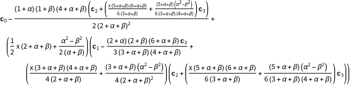
Evaluate a finite Jacobi sum with symbolic coefficients and parameters:
| In[3]:= |
|
| Out[3]= |
|
Compare with an explicit summation:
| In[4]:= |
|
| Out[4]= |
|
Evaluate a partial sum of a Gegenbauer series:
| In[5]:= |
|
| Out[5]= |
|
Compare with an explicit summation:
| In[6]:= |
|
| Out[6]= |
|
Evaluate a finite Hermite sum with coefficients supplied from a list:
| In[7]:= |
|
| Out[7]= |
|
Compare with an explicit evaluation:
| In[8]:= |
|
| Out[8]= |
|
Generate random coefficients of a Legendre series:
| In[9]:= |
|
Evaluating the Legendre series with OrthogonalPolynomialSum is faster than using LegendreP:
| In[10]:= |
|
| Out[10]= |
|
| In[11]:= |
|
| Out[11]= |
|
The result obtained through OrthogonalPolynomialSum also has a slightly smaller error:
| In[12]:= |
|
| Out[12]= |
|
| In[13]:= |
|
| Out[13]= |
|
| In[14]:= |
|
| Out[14]= |
|
This work is licensed under a Creative Commons Attribution 4.0 International License