Details and Options
If
points is given as a numeric
List, the values are taken to be in micrometers.
ResourceFunction["OpticalFieldModeling"] takes the following options:
| "CoherenceFunction" | None | calculates the phase of every real point light source |
| "PhaseFunction" | None | calculates the complex degree of spatial coherence of every virtual point |
"PhaseFunction" is supplied with the coordinates of each real point and should return a numerical value in radians.
With the default setting
"PhaseFunction"→None, the phase value of every real point is set to 0, representing a plane wavefront.
"CoherenceFunction" is supplied with the distance vector of every length-two subset of real points and should return a numerical value between 0 and 1.
With the default setting
"CoherenceFunction"→None, the coherence value of every virtual point is set to 1, representing a fully spatially coherent light source.
The PointArrayObject expression returned by ResourceFunction["OpticalFieldModeling"] supports the following properties:
| "PointPlot" | a plot showing the locations of the real points and their corresponding virtual points |
| "PowerSpectrum" | a PowerSpectrumObject based on the given wavelength and propagation distance |
The "PowerSpectrum" property requires the arguments λ (wavelength) and z (propagation distance): PointArrayObject[…]["PowerSpectrum",λ,z].
The
"PointPlot" property of
PointArrayObject accepts the same options as the
NumberLinePlot (for 1D point arrays) or
ListPlot (for 2D point arrays) functions.
The PowerSpectrumObject expression returned by the "PowerSpectrum" property of a PointArrayObject supports the following properties:
| "Expression" | complete power spectrum expression |
| "Plot" | power spectrum 1D plot along the horizontal axis |
| "DensityPlot" | power spectrum density plot |
The "Plot" and "DensityPlot" properties accept arguments for angle (in degrees) and plotting step: PowerSpectrumObject[…]["Plot",angle,step].
The
angle specifies the maximum half-angle of the cone of light. If unspecified or set to
Automatic,
angle is taken by default to be 65°.
If unspecified or set to
Automatic,
step is calculated based on a fraction of the propagation distance of the
PowerSpectrumObject.
The
"Plot" and
"DensityPlot" properties of
PowerSpectrumObject accept the same options as the
ListPlot and
DensityPlot functions.

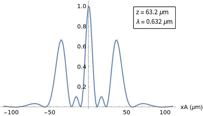
![\[Lambda] = 0.632;
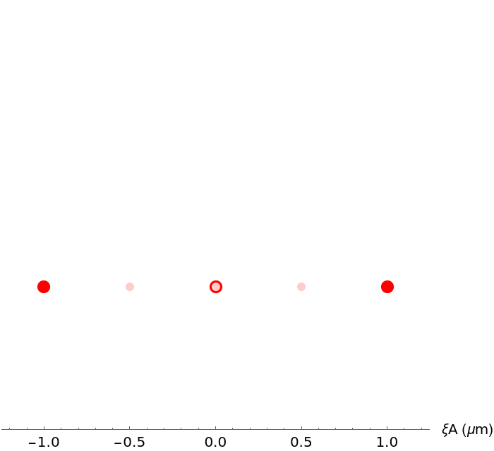
pointArray1D = ResourceFunction["OpticalFieldModeling"][
N@Range[-2 \[Lambda], 2 \[Lambda], 2 \[Lambda]]];
powerSpectrum1D = pointArray1D["PowerSpectrum", \[Lambda], 100 \[Lambda]];
powerSpectrum1D["Plot", 60, 1.6]](https://www.wolframcloud.com/obj/resourcesystem/images/80a/80a2b21e-f85b-4976-a29e-0210c39ccea0/5a87acb1032e622c.png)


![\[Sigma] = 2;
coherenceF[\[Xi]D_] := N@Exp[-\[Xi]D^2/(2 \[Sigma]^2)];
ResourceFunction["OpticalFieldModeling"][Range[-3, 3], "CoherenceFunction" -> coherenceF]](https://www.wolframcloud.com/obj/resourcesystem/images/80a/80a2b21e-f85b-4976-a29e-0210c39ccea0/6fa9bc3a736034d2.png)

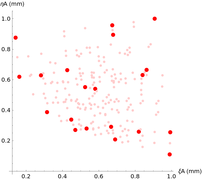
![\[Sigma] = 2000;
ResourceFunction["OpticalFieldModeling"][
QuantityArray[RandomReal[3, {5, 2}], "Millimeters"], "CoherenceFunction" -> (Exp[-((#1^2 + #2^2)/(2 \[Sigma]^2))] &)]](https://www.wolframcloud.com/obj/resourcesystem/images/80a/80a2b21e-f85b-4976-a29e-0210c39ccea0/394520e55674524e.png)


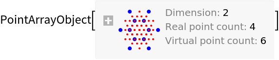
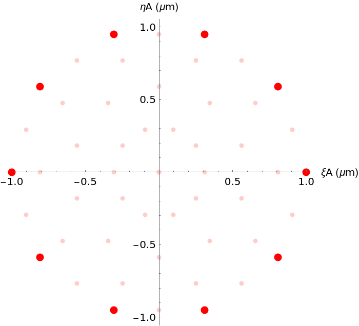
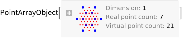
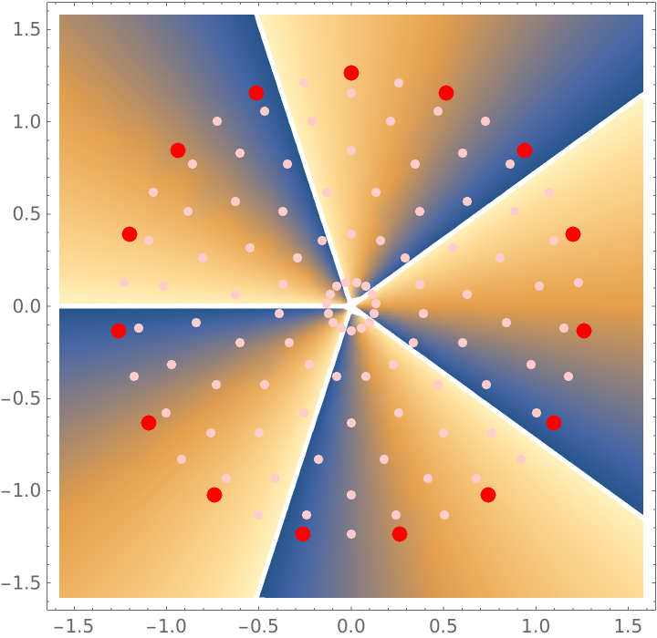
![m = 5;
vortexPointArray = ResourceFunction["OpticalFieldModeling"][
N@CirclePoints[2 \[Lambda], 15], "PhaseFunction" -> Function[{\[Xi]A, \[Eta]A}, Mod[m ArcTan[\[Xi]A, \[Eta]A] + \[Pi], 2 \[Pi]]]]](https://www.wolframcloud.com/obj/resourcesystem/images/80a/80a2b21e-f85b-4976-a29e-0210c39ccea0/136bdcf1ddea560d.png)

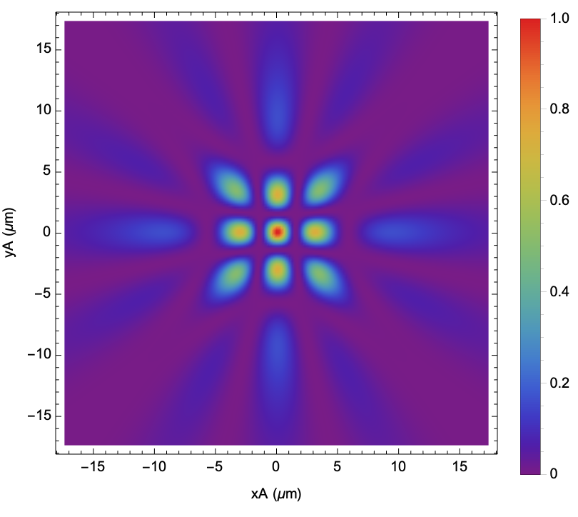
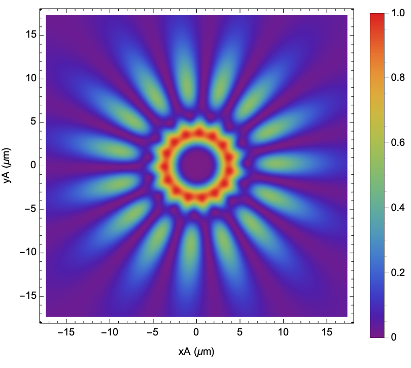
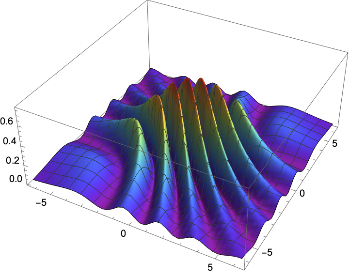
![\[Lambda] = 0.632;
z = 10 \[Lambda];
vortexPowerSpectrum = vortexPointArray["PowerSpectrum", \[Lambda], z];
vortexPowerSpectrum["DensityPlot", 70, z/40]](https://www.wolframcloud.com/obj/resourcesystem/images/80a/80a2b21e-f85b-4976-a29e-0210c39ccea0/6c66b5fe8569904f.png)
![\[Sigma] = 4 \[Lambda]; gratingPointArray = ResourceFunction["OpticalFieldModeling"][
Flatten[Table[{i, 0}, {i, -6 \[Lambda], 6 \[Lambda], 2 \[Lambda]}, {j, 1}], 1], "CoherenceFunction" -> Function[{\[Xi]D, \[Eta]D}, E^(-(\[Xi]D^2 + \[Eta]D^2)/(
2 \[Sigma]^2))]]](https://www.wolframcloud.com/obj/resourcesystem/images/80a/80a2b21e-f85b-4976-a29e-0210c39ccea0/1d174628d3ee3dae.png)

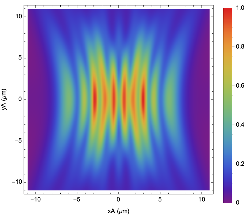
![\[Lambda] = 0.632;
z - 10 \[Lambda];
gratingPowerSpectrum = gratingPointArray["PowerSpectrum", \[Lambda], z];
gratingPowerSpectrum["DensityPlot", 60, z/40]](https://www.wolframcloud.com/obj/resourcesystem/images/80a/80a2b21e-f85b-4976-a29e-0210c39ccea0/60535a593d41d0e3.png)
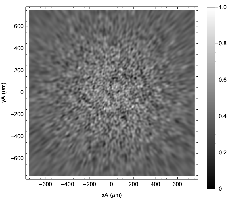
![phaseF[\[Xi]A_, \[Eta]A_] := RandomReal[{-\[Pi], \[Pi]}]; \[Lambda] = 0.632;
speckleArray = ResourceFunction["OpticalFieldModeling"][
RandomPoint[Disk[{0, 0}, 20 \[Lambda]], 150], "PhaseFunction" -> phaseF];
specklePS = speckleArray["PowerSpectrum", \[Lambda], 1000 \[Lambda]];
specklePS["DensityPlot", 50, ColorFunction -> GrayLevel]](https://www.wolframcloud.com/obj/resourcesystem/images/80a/80a2b21e-f85b-4976-a29e-0210c39ccea0/64be246032b03639.png)
![\[Lambda] = 520; z = 10 \[Lambda];
ResourceFunction["OpticalFieldModeling"][
QuantityArray[RandomReal[1, {20, 2}], "Millimeters"], Quantity[\[Lambda], "Nanometers"], Quantity[z, "Micrometers"]]](https://www.wolframcloud.com/obj/resourcesystem/images/80a/80a2b21e-f85b-4976-a29e-0210c39ccea0/3b6a5e6fd69e2427.png)

![\[Lambda] = 0.632;
pointArray = ResourceFunction["OpticalFieldModeling"][{{-1, -1}, {1, 1}}];
powerSpectrum = pointArray["PowerSpectrum", \[Lambda], 5 \[Lambda]];
powerSpectrum["Expression"]](https://www.wolframcloud.com/obj/resourcesystem/images/80a/80a2b21e-f85b-4976-a29e-0210c39ccea0/7998a7e790955682.png)

![\[Sigma] = 20;
ResourceFunction["OpticalFieldModeling"][
QuantityArray[RandomReal[3, {5, 2}], "Millimeters"], "CoherenceFunction" -> (Exp[-((#1^2 + #2^2)/(2 \[Sigma]^2))] &)]](https://www.wolframcloud.com/obj/resourcesystem/images/80a/80a2b21e-f85b-4976-a29e-0210c39ccea0/6610fcb58157bf98.png)
