Wolfram Function Repository
Instant-use add-on functions for the Wolfram Language
Function Repository Resource:
A statistical distribution for the sum of a normal and an asymmetric Laplace random variable
ResourceFunction["NormalLaplaceDistribution"][α,β,μ,σ] represents a normal Laplace distribution. |
Define and compute the mean of a normal Laplace distribution:
| In[1]:= |
| Out[2]= |
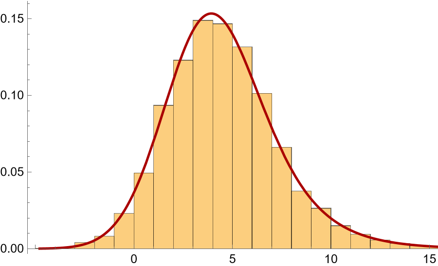
Generate a random sample and fit it to the NormalLaplaceDistribution:
| In[3]:= | ![{a, b, d, c} = {0.5, 2, 3, 2};
s = RandomVariate[
ResourceFunction["NormalLaplaceDistribution"][a, b, d, c], 10000];
h0 = Histogram[s, Automatic, "PDF"];
g1 = Plot[
PDF[ResourceFunction["NormalLaplaceDistribution"][a, b, d, c], x], {x, Min[s], Max[s]}, PlotRange -> All, PlotStyle -> {Thick, Darker[Red]}];
Show[h0, g1]](https://www.wolframcloud.com/obj/resourcesystem/images/25d/25d4f22c-1bce-4ff2-b34b-8a4b5458e4fa/65122dbec6d6d887.png) |
| Out[4]= |  |
Estimate the distribution from this sample:
| In[5]:= |
| Out[5]= |
Display the distribution parameters:
| In[6]:= |
| Out[6]= |
The distribution can be used with other statistical functions, for example estimate the mean with parameters:
| In[7]:= |
| Out[7]= |
StandardDeviation estimate with parameters:
| In[8]:= |
| Out[8]= |
The characteristic function of the NormalLaplaceDistribution:
| In[9]:= |
| Out[9]= |  |
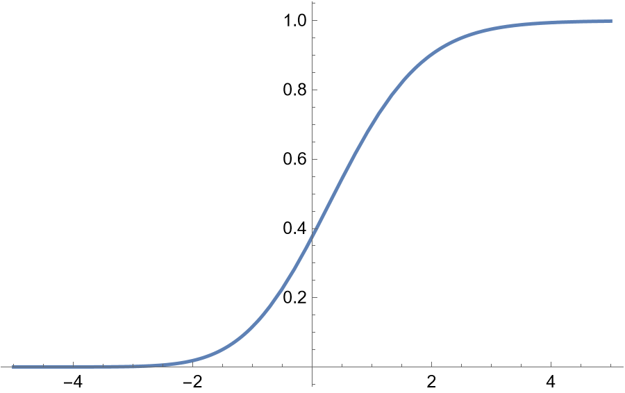
Plot the distribution function for a given set of parameter values:
| In[10]:= |
| Out[10]= |  |
The Quantile function is listable:
| In[11]:= |
| Out[11]= |
The CDF is also listable:
| In[12]:= |
| Out[12]= |
The NormalLaplaceDistribution is the distribution of the sum of random variables from a NormalDistribution and the difference of two ExponentialDistribution random variables. Start with the TransformedDistribution:
| In[13]:= |
| Out[13]= |
When the PDF is requested from the output above the full formula for the density is computed:
| In[14]:= |
| Out[14]= |
Check equivalence:
| In[15]:= |
| Out[15]= |
Here the characteristic function of the transformed distribution is computed:
| In[16]:= |
| Out[16]= |  |
Check equivalence:
| In[17]:= |
| Out[17]= |
Wolfram Language 13.0 (December 2021) or above
This work is licensed under a Creative Commons Attribution 4.0 International License