Wolfram Function Repository
Instant-use add-on functions for the Wolfram Language
Function Repository Resource:
Decompose a matrix into two non-negative matrix factors
ResourceFunction["NonNegativeMatrixFactorization"][mat,k] finds non-negative matrix factors for the matrix mat using k dimensions. |
| "Epsilon" | 10-9 | denominator (regularization) offset |
| MaxSteps | 200 | maximum iteration steps |
| "NonNegative" | True | should the non-negativity be enforced at each step |
| "Normalization" | Left | which normalization is applied to the factors |
| PrecisionGoal | Automatic | precision goal |
| "ProfilingPrints" | False | should profiling times be printed out during execution |
| "RegularizationParameter" | 0.01 | regularization (multiplier) parameter |
Create a random integer matrix:
| In[1]:= | ![SeedRandom[7]
mat = RandomInteger[10, {4, 3}];
MatrixForm[mat]](https://www.wolframcloud.com/obj/resourcesystem/images/546/546fd07f-c179-4cfe-ad49-58aeaf49babb/41ce7c2d1134183c.png) |
| Out[3]= |  |
Compute the NNMF factors:
| In[4]:= |
| Out[4]= |  |
Here is the matrix product of the obtained factors:
| In[5]:= |
| Out[8]= |  |
Note that elementwise relative errors between the original matrix and reconstructed matrix are small:
| In[9]:= |
| Out[12]= |  |
Here is a random matrix with its first two columns having much larger magnitudes than the rest:
| In[13]:= | ![SeedRandom[278];
mat = RandomReal[{20, 100}, {10, 2}];
mat2 = RandomReal[{10, 30}, {10, 7}];
mat = ArrayPad[mat, {{0, 0}, {0, 5}}] + mat2;
ListLinePlot[Transpose[mat], PlotRange -> All, ImageSize -> Medium, PlotTheme -> "Detailed"]](https://www.wolframcloud.com/obj/resourcesystem/images/546/546fd07f-c179-4cfe-ad49-58aeaf49babb/6a78680bba944cfe.png) |
| Out[13]= | 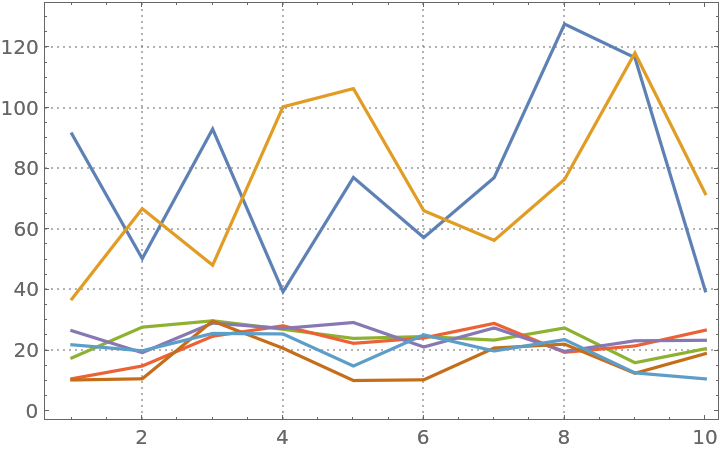 |
Here we compute NNMF factors:
| In[14]:= |
Find the relative error of the approximation by the matrix factorization:
| In[15]:= |
| Out[15]= |
Here is the relative error for the first three columns:
| In[16]:= |
| Out[16]= |
Here are comparison plots:
| In[17]:= | ![Block[{opts = {PlotRange -> All, ImageSize -> 250, PlotTheme -> "Detailed"}}, Row[{ListLinePlot[Transpose[mat], opts, PlotLabel -> "Orginal"], ListLinePlot[Transpose[W . H], opts, PlotLabel -> "Reconstructed"]}]]](https://www.wolframcloud.com/obj/resourcesystem/images/546/546fd07f-c179-4cfe-ad49-58aeaf49babb/2b37ac768f6878dc.png) |
| Out[17]= | 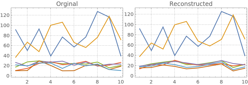 |
NNMF factors can be normalized in two ways: (i) the Euclidean norms of the columns of the left factor are all equal to 1; or (ii) the Euclidean norms of the rows of the right factor are all equal to 1. Here is a table that shows NNMF factors for different normalization specifications:
| In[18]:= | ![Block[{mat},
SeedRandom[7];
mat = RandomInteger[10, {4, 3}];
Multicolumn[
Table[
SeedRandom[121];
{W, H} = ResourceFunction["NonNegativeMatrixFactorization"][mat, 2, "Normalization" -> nspec];
Grid[{
{Style[nspec, Bold, Blue], SpanFromLeft},
{Labeled[MatrixForm[W], "W", Top], Labeled[MatrixForm[H], "H", Top]},
{"Norm/@Transpose[W]:", Norm /@ Transpose[W]},
{"Norm/@H:", Norm /@ H}},
Dividers -> All, FrameStyle -> GrayLevel[0.8], Alignment -> Left
], {nspec, {Automatic, Left, Right, True, False, None}}],
2, Dividers -> All]
]](https://www.wolframcloud.com/obj/resourcesystem/images/546/546fd07f-c179-4cfe-ad49-58aeaf49babb/3c0d56cdd773e7ac.png) |
| Out[18]= | 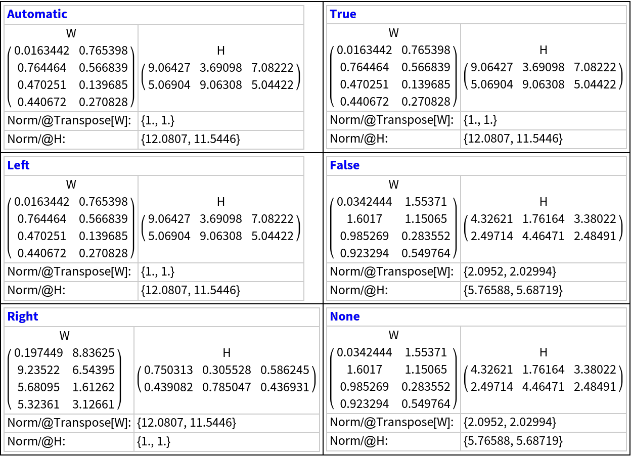 |
The implemented NNMF algorithm uses the gradient descent algorithm. The regularization parameter controls the “learning rate” and can have dramatic influence on the number of iteration steps and approximation precision. Compute NNMF with different regularization multiplier parameters:
| In[19]:= | ![res = Association[# -> BlockRandom[SeedRandom[22];
ResourceFunction["NonNegativeMatrixFactorization"][mat, 3, "RegularizationParameter" -> #, MaxSteps -> 10, PrecisionGoal -> 3]] & /@ {0.01, 2}];](https://www.wolframcloud.com/obj/resourcesystem/images/546/546fd07f-c179-4cfe-ad49-58aeaf49babb/00ab77aae1832488.png) |
Plot the results:
| In[20]:= | ![Grid[KeyValueMap[{#1, ListLinePlot[Transpose[#2[[1]]], PlotRange -> All, ImageSize -> 250, PlotTheme -> "Detailed"]} &, res], Alignment -> {Center, Left}]](https://www.wolframcloud.com/obj/resourcesystem/images/546/546fd07f-c179-4cfe-ad49-58aeaf49babb/76fbdff5ee7eb3df.png) |
| Out[20]= | 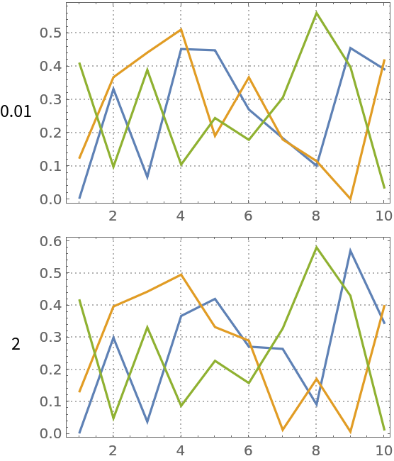 |
Here are the corresponding norms:
| In[21]:= |
| Out[21]= |
One of the main motivations for developing NNMF algorithms is the easier interpretation of extracted topics in the framework of latent semantic analysis. The following code illustrates the extraction of topics over a dataset of movie reviews.
Start with a movie reviews dataset:
| In[22]:= |
| Out[22]= |
Change the labels “positive” and “negative” to have the prefix “tag:”:
| In[23]:= |
Concatenate to each review the corresponding label and create an Association:
| In[24]:= | ![aMovieReviews = AssociationThread[
Range[Length[movieReviews]] -> Map[StringRiffle[List @@ #, " "] &, movieReviews]];
RandomSample[aMovieReviews, 2]](https://www.wolframcloud.com/obj/resourcesystem/images/546/546fd07f-c179-4cfe-ad49-58aeaf49babb/3b4171045d9710a9.png) |
| Out[24]= |  |
Select movie reviews that are nontrivial:
| In[25]:= |
| Out[25]= |
Split each review into words and delete stopwords:
| In[26]:= |
Convert the movie reviews association into a list of ID-word pairs (“long form”):
| In[27]:= | ![lsLongForm = Join @@ MapThread[Thread[{##}] &, Transpose[List @@@ Normal[aMovieReviews2]]];
RandomSample[lsLongForm, 4]](https://www.wolframcloud.com/obj/resourcesystem/images/546/546fd07f-c179-4cfe-ad49-58aeaf49babb/246a87048cdedb25.png) |
| Out[27]= |
Replace each word with its Porter stem:
| In[28]:= | ![AbsoluteTiming[
aStemRules = Dispatch[
Thread[Rule[#, WordData[#, "PorterStem"] & /@ #]] &@
Union[lsLongForm[[All, 2]]]];
lsLongForm[[All, 2]] = lsLongForm[[All, 2]] /. aStemRules;
]](https://www.wolframcloud.com/obj/resourcesystem/images/546/546fd07f-c179-4cfe-ad49-58aeaf49babb/0fdc54ac0f2ea2d7.png) |
| Out[28]= |
Find the frequency of appearance of all unique word stems and pick words that appear in more than 30 reviews:
| In[29]:= | ![aTallies = Association[Rule @@@ Tally[lsLongForm[[All, 2]]]];
aTallies = Select[aTallies, # > 20 &];
Length[aTallies]](https://www.wolframcloud.com/obj/resourcesystem/images/546/546fd07f-c179-4cfe-ad49-58aeaf49babb/64494bf3b4575cd0.png) |
| Out[29]= |
Filter the ID-word pairs list to contain only words that are sufficiently popular:
| In[30]:= |
Compute an ID-word contingency matrix:
| In[31]:= |
Here is a sample of the contingency matrix as a dataset:
| In[32]:= |
| Out[32]= | 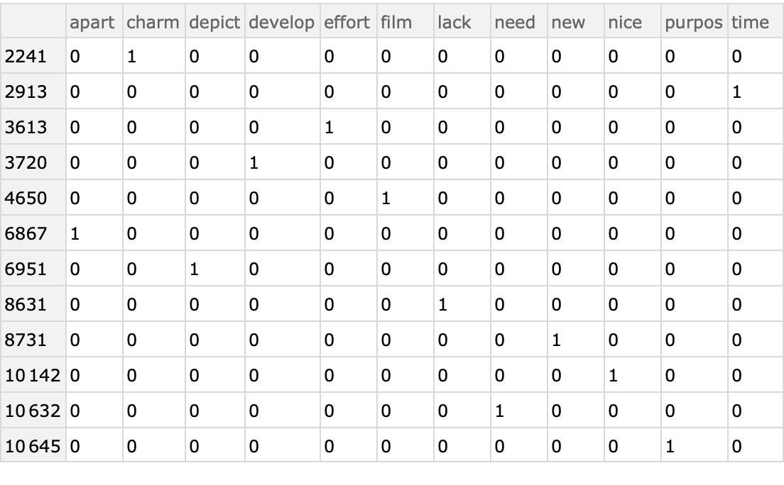 |
Visualize the contingency matrix:
| In[33]:= | ![CTMatrixPlot[x_Association /; KeyExistsQ[x, "SparseMatrix"], opts___] := MatrixPlot[x["SparseMatrix"], Append[{opts}, FrameLabel -> {{Keys[x][[2]], None}, {Keys[x][[3]], None}}]];
CTMatrixPlot[ctObj]](https://www.wolframcloud.com/obj/resourcesystem/images/546/546fd07f-c179-4cfe-ad49-58aeaf49babb/59e7df3d538610bf.png) |
| Out[33]= | 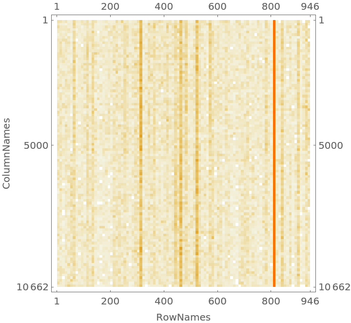 |
Take the contingency sparse matrix:
| In[34]:= |
Here is a plot generated by the resource function ParetoPrinciplePlot that shows the Pareto principle adherence of the selected popular words:
| In[35]:= |
| Out[35]= | 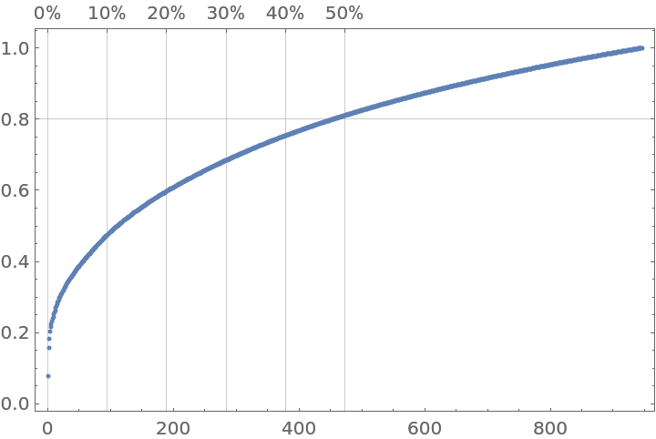 |
Judging from the Pareto plot we should apply the inverse document frequency (IDF) formula:
| In[36]:= |
Normalize each row with the Euclidean norm:
| In[37]:= |
In order to get computations faster, we take a sample submatrix:
| In[38]:= |
| Out[38]= |
Apply NNMF in order to extract 24 topics using 12 maximum iteration steps, normalizing the right factor:
| In[39]:= | ![SeedRandom[23];
AbsoluteTiming[
{W, H} = ResourceFunction["NonNegativeMatrixFactorization"][matCT2, 24, MaxSteps -> 12, "Normalization" -> Right];
]](https://www.wolframcloud.com/obj/resourcesystem/images/546/546fd07f-c179-4cfe-ad49-58aeaf49babb/3fa1a903e31419ab.png) |
| Out[39]= |
Show the extracted topics using the right factor (H):
| In[40]:= | ![Multicolumn[
Table[
Column[{Style[ind, Blue, Bold], ColumnForm[
Keys[TakeLargest[
AssociationThread[
ctObj["ColumnNames"] -> Normal[H[[ind, All]]]], 10]]]}],
{ind, Dimensions[H][[1]]}
], 8, Dividers -> All]](https://www.wolframcloud.com/obj/resourcesystem/images/546/546fd07f-c179-4cfe-ad49-58aeaf49babb/631adfdac4a4479d.png) |
| Out[40]= | 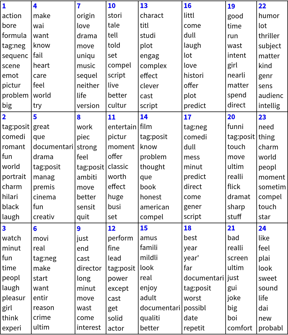 |
Here we show statistical thesaurus entries for random words, selected words and the labels (“tag:positive”,”tag:negative”):
| In[41]:= | ![SeedRandom[898];
rinds = Flatten[
Position[ctObj["ColumnNames"], #] & /@ Map[WordData[#, "PorterStem"] &, {"tag:positive", "tag:negative", "book", "amusing", "actor", "plot", "culture", "comedy", "director", "thoughtful", "epic", "film", "bad", "good"}]];
rinds = Sort@
Join[rinds, RandomSample[Range[Dimensions[H][[2]]], 16 - Length[rinds]]];
Multicolumn[
Table[
Column[{Style[ctObj["ColumnNames"][[ind]], Blue, Bold], ColumnForm[
ctObj["ColumnNames"][[
Flatten@Nearest[Normal[Transpose[H]] -> "Index", H[[All, ind]], 12]]]]}],
{ind, rinds}
], 8, Dividers -> All]](https://www.wolframcloud.com/obj/resourcesystem/images/546/546fd07f-c179-4cfe-ad49-58aeaf49babb/4a1c13ebec224ddd.png) |
| Out[41]= | 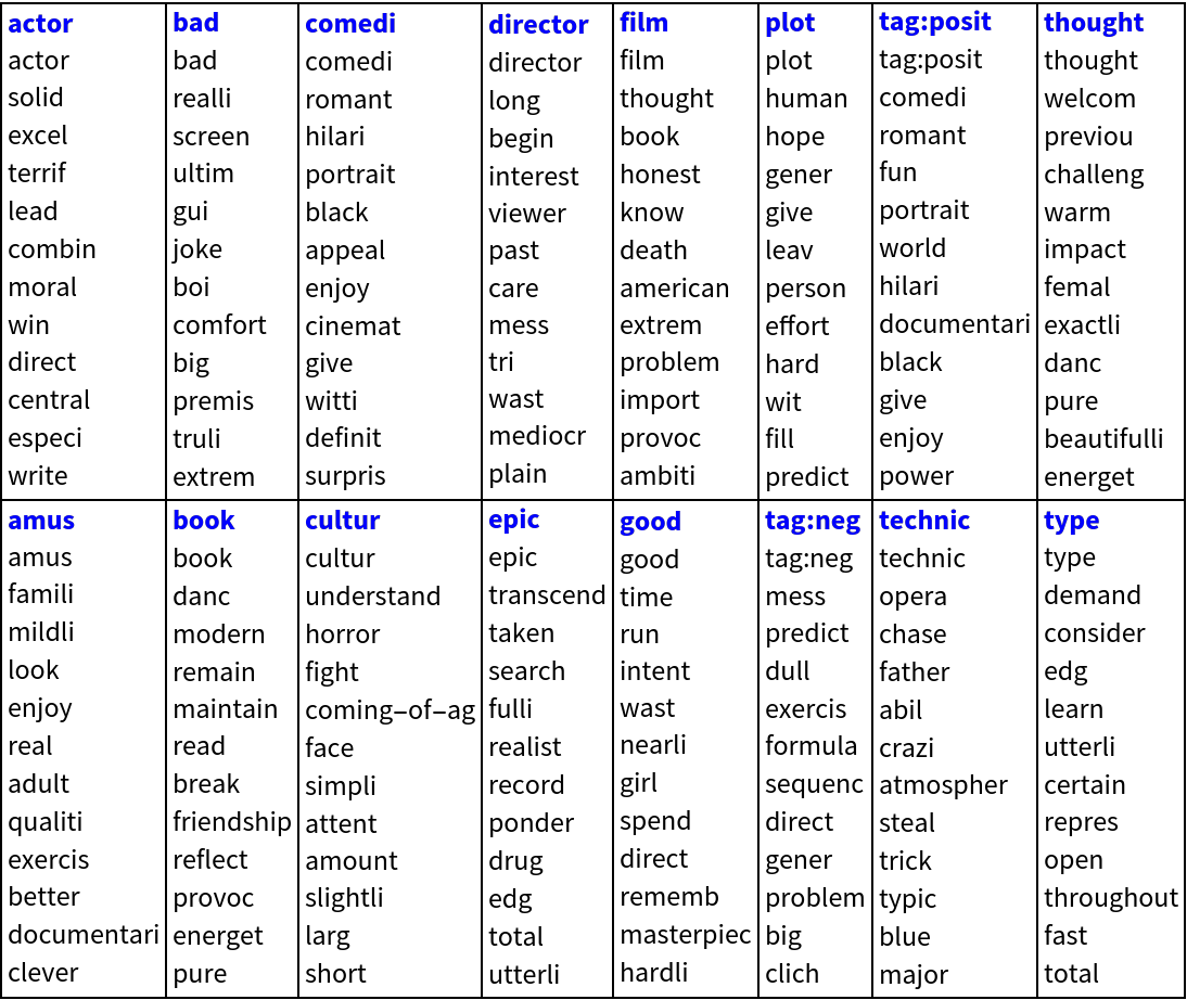 |
NNMF should be compared with the singular value decomposition (SVD) and independent component analysis (ICA).
Generate 3D points:
| In[42]:= | ![n = 200;
c = 12;
SeedRandom[232];
points = Transpose[
RandomVariate[NormalDistribution[0, #], n] & /@ {2, 4, 0.1}];
points = points . RotationMatrix[{{0, 0, 1}, {-1, 0, 1}}];
points = Map[{2, 8, 2} + # &, points];
points = Clip[points, {0, Max[points]}];
opts = {BoxRatios -> {1, 1, 1}, PlotRange -> Table[{c, -c}, 3], FaceGrids -> {{0, 0, -1}, {0, 1, 0}, {-1, 0, 0}}, ViewPoint -> {-1.1, -2.43, 2.09}};
gr0 = ListPointPlot3D[points, opts];](https://www.wolframcloud.com/obj/resourcesystem/images/546/546fd07f-c179-4cfe-ad49-58aeaf49babb/339913a9ce600d8e.png) |
Compute matrix factorizations using NNMF, SVD and ICA and make a comparison plots grid (rotate the graphics boxes for better perception):
| In[43]:= | ![SeedRandom[232];
{W, H} = ResourceFunction["NonNegativeMatrixFactorization"][points, 2, "Normalization" -> Right];
grNNMF = Show[{ListPointPlot3D[points], Graphics3D[{Red, Arrow[{{0, 0, 0}, #}] & /@ (c*H/Norm[H])}]}, opts, PlotLabel -> "NNMF"];
{U, S, V} = SingularValueDecomposition[points, 2];
grSVD = Show[{ListPointPlot3D[points], Graphics3D[{Red, Arrow[{{0, 0, 0}, #}] & /@ (c*Transpose[V])}]}, opts, PlotLabel -> "SVD"];
{A, S} = ResourceFunction["IndependentComponentAnalysis"][points, 2];
grICA = Show[{ListPointPlot3D[points], Graphics3D[{Red, Arrow[{{0, 0, 0}, #}] & /@ (c*S/Norm[S])}]}, opts, PlotLabel -> "ICA"];
Grid[{{gr0, grSVD}, {grICA, grNNMF}}]](https://www.wolframcloud.com/obj/resourcesystem/images/546/546fd07f-c179-4cfe-ad49-58aeaf49babb/596ecdd82b0a23d4.png) |
| Out[43]= | 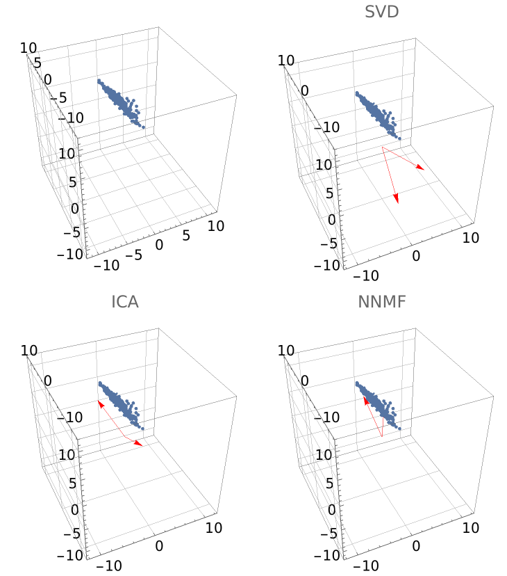 |
This work is licensed under a Creative Commons Attribution 4.0 International License