Basic Examples (2) 

Compute entropy for a nearest neighbor graph of 20 random points:

In[1]:=

Out[1]=

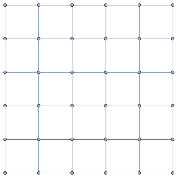
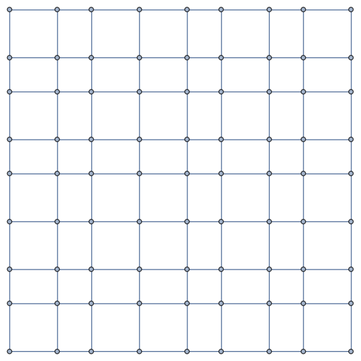
Build the nearest neighbor graph of a perfect square lattice with unit lattice constant:

In[2]:=

Out[3]=

In[4]:=

Out[4]=

Compute the graph entropy and verify it is equal to zero as expected by symmetry:

In[5]:=

Out[5]=

Scope (3) 

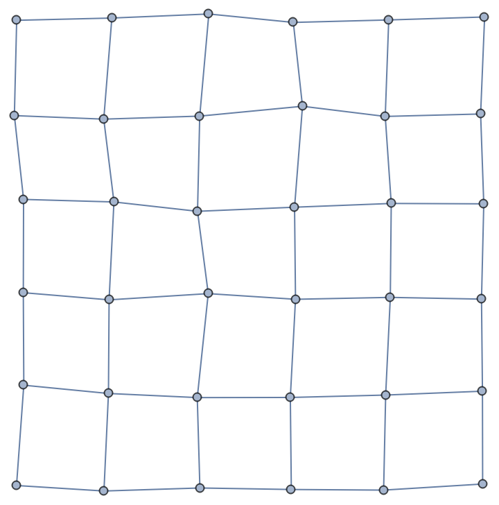
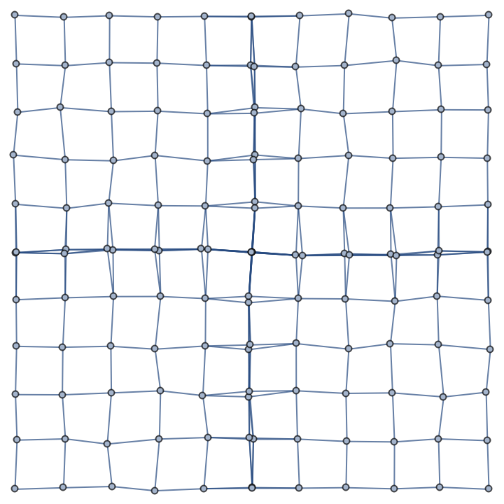
Define a 2D set of point arranged in a square lattice, add distortions to have all edges unequal as in a 2D disordered system and build the corresponding NearestNeighborGraph with all nearest neighbor connections within a given radius:

In[6]:=

Out[9]=

Compute the graph entropy:

In[10]:=

Out[10]=

Check it is equal to the natural logarithm of the number of distinct edges in the graph:

In[11]:=

Out[11]=

Options (2) 

Treat some distance values as equal if they differ by an optional threshold "MinThreshold" set to a given positive value. This introduces some order into the graph layout:

In[12]:=

In[13]:=

In[14]:=

Out[14]=

Check that graph entropy is lower than in the case without rounding factor:

In[15]:=

Out[15]=

Applications (2) 

Build a linear graph mapped to the coordinates of a one-dimensional Fibonacci quasiperiodic chain with nit iterations and spacing ratio between nodes tau:

In[16]:=

In[17]:=

Out[17]=

Computes its graph entropy:

In[18]:=

Out[18]=

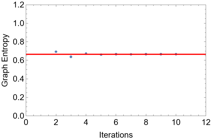
Check that the numerical value of the graph entropy converges to the universal value 0.665:

In[19]:=

Out[19]=

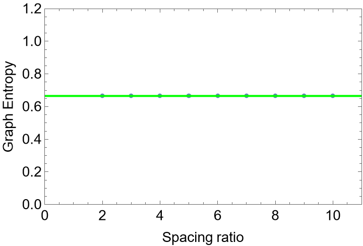
This universal value 0.665 is also independent of the spacing ratio between graph nodes:

In[20]:=

Out[20]=

If a point symmetry element of order C_n is present in the graph, then the graph entropy is equal to ln(E/n) where E is the total number of edges in the graph and n is the order of the rotation symmetry.

Start from a slightly disordered square lattice and apply rotations of 0, π/2, π and -π/2 to the starting lattice points to get three additional sub-lattices:

In[21]:=

Build the overall graph connecting all points belonging to the four sub-lattices:

In[22]:=

Out[22]=

Compute numerically the graph entropy for this system:

In[23]:=

Out[23]=

Check that it is close to the natural logarithm of the number of graph edges divided by the symmetry order:

In[24]:=

Out[24]=

Properties and Relations (2) 

Define a grid of points:

In[25]:=

Out[25]=

As noise is added to the graph, the entropy increases:

In[26]:=

Out[26]=

Neat Examples (2) 

Build a 2D graph mapped to the coordinates of a two-dimensional Fibonacci quasiperiodic array with nit iterations:

In[27]:=

In[28]:=

Out[28]=

In[29]:=

Out[29]=

Check that the numerical value of the graph entropy still converges to the universal value 0.665 known from 1D case (computation takes a few seconds):

In[30]:=

Out[30]=

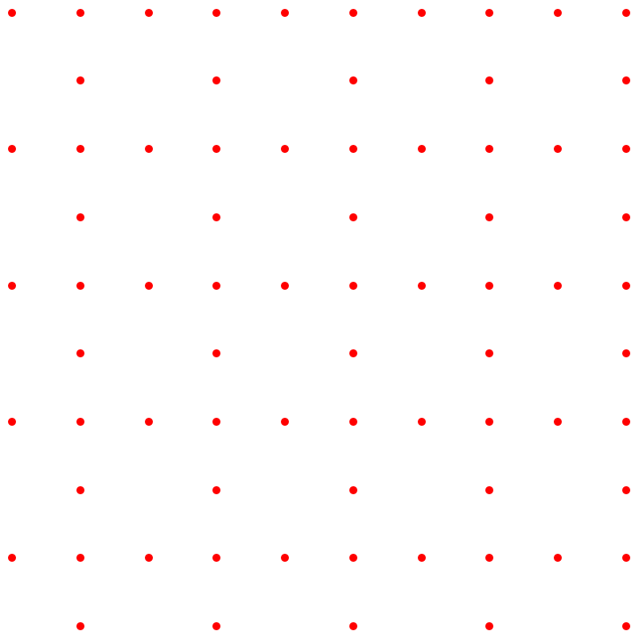
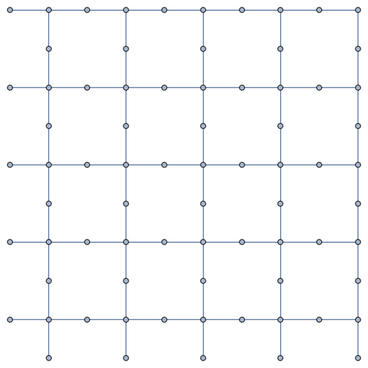
A semi-regular set of points obtained by alternatively deleting sites from a square lattice:

In[31]:=

Out[4]=

In[32]:=

Out[32]=

Check that the graph entropy is still zero as expected by symmetry:

In[33]:=

Out[33]=