Basic Examples (2)
Numerically solve a univariate polynomial equation in x:
Numerically solve a multivariate system of polynomial equations:
Scope (7)
Create a real-valued polynomial objective function f in three variables x, y, z using random coefficient parameters:
Find stationary points of the objective f:
Select the real valued ones:
Function values at these critical points:
Sorted critical points according to the function value:
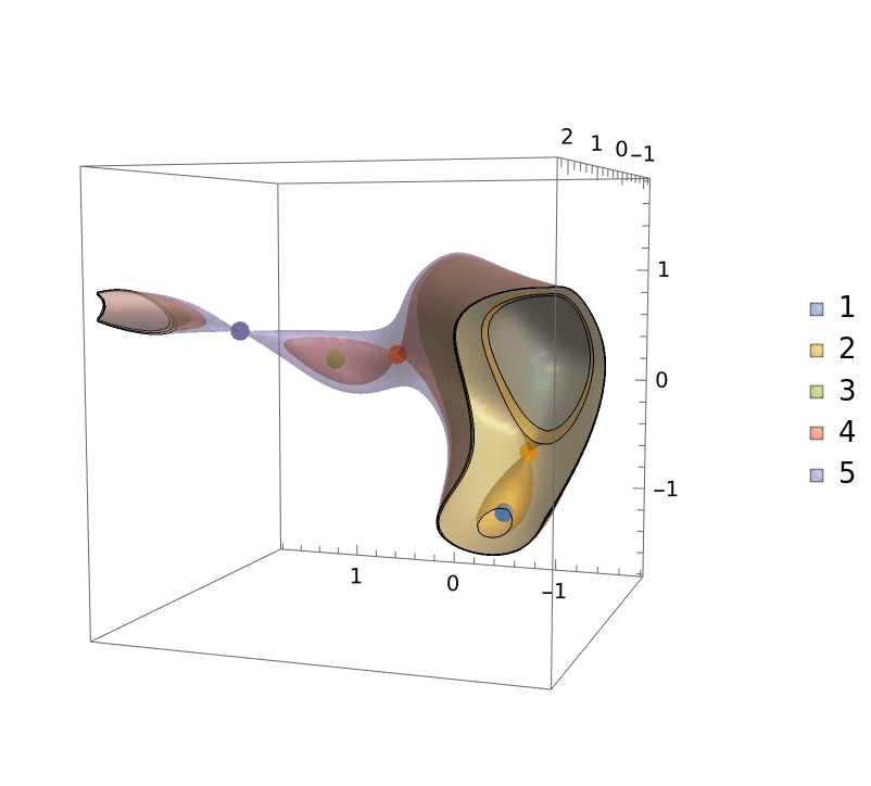
Two of these (namely, #1 and #3) are local minima with all positive eigenvalues of the local Hessian, while the rest are saddle points:
Local minima and saddle points can be also discerned via the following ContourPlot3D visualization:
Options (3)
Default execution may not find all isolated roots:
All the roots may be obtained by increasing or decreasing "Radius" parameter:
"MaxRoots" can be used to compute a subset of the total roots for unwieldy polynomial systems:
Generate a random large polynomial system of dimension 5 and total degree 100,000:
Compute 50 roots:
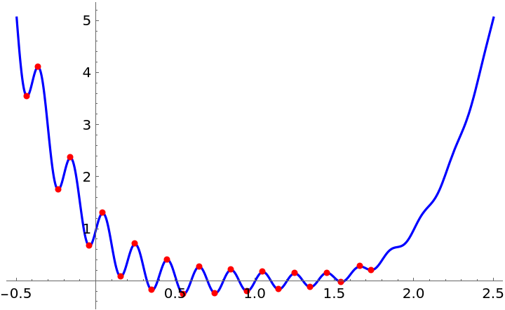
In some cases transcendental functions can be minimized using "MaxRoots" termination criterion:
Visualize the real valued stationary points:
Properties and Relations (5)
NSolveByMonodromy can find many or all of the isolated roots with or without an initial point, e.g., a bifurcation problem:
FindRoot attempts to find one root at a time based on an initial point:
NSolveByMonodromy compares favorably against NSolve in some large systems, e.g., 6R inverse position kinematics:
NSolve default execution is 4 times slower and returns duplicate instances requiring an additional filtration step to remove them:
NSolve execution in high-precision takes even longer than the default execution:
Another example, a reduced 8-dimensional system arising in economics:
NSolve default execution misses two isolated roots and returns some duplicate instances instead:
NSolve in high-precision returns the correct set of roots in a comparable time with NSolveByMonodromy:
NSolveByMonodromy does not accept a search range as input, unlike NSolve:
Select the real valued ones:
NSolve solves this system if a search range is provided:
NSolveByMonodromy can only solve square systems:
NSolve computes some witness points for such under-determined systems:
Possible Issues (2)
NSolveByMonodromy cannot solve non-analytic systems:
NSolve solves this system using inverse functions:
NSolveByMonodromy may fail to proceed beyond initial point in systems with special monomial structures and/or parameters:
NSolve finds the approximation of all the 20 roots for the Wilkinson's polynomial:
Neat Examples (6)
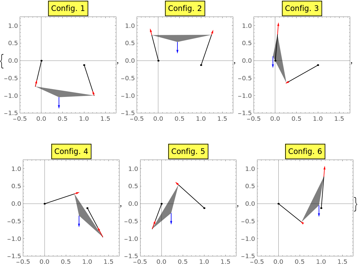
Static equilibria of a weight suspended by two massless cables, each of different given lengths, in a plane:
This 10-dimensional system admits 12 nonsingular isolated roots in a generic case, as found by NSolveByMonodromy:
NSolve default execution takes a long time:
The presence of singular and positive-dimensional sets impacts the results of NSolve:
Select the real valued ones in x, y:
Visualize the real equilibria, in which Configuration 1 is the only stable one with both cables under tension:
![SeedRandom[1234];
ResourceFunction["NSolveByMonodromy"][x^2 + 5 x + 6, x]](https://www.wolframcloud.com/obj/resourcesystem/images/372/3722b78e-6f4f-4a85-b103-cbf5004da4c5/139575fb611b537c.png)
![eqns = {45*P + 35*S - 165*B - 36, 35*P + 40*Z + 25*T - 27*S, 15*W + 25*P*S + 30*Z - 18*T - 165*B^2, -9*W + 15*P*T + 20*Z*S, W*P + 2*Z*T - 11*B^3, 99*W - 11*S*B + 3*B^2};
vars = {P, S, B, Z, T, W};
solns = ResourceFunction["NSolveByMonodromy"][eqns, vars];
solns // Length](https://www.wolframcloud.com/obj/resourcesystem/images/372/3722b78e-6f4f-4a85-b103-cbf5004da4c5/7be579248cb71c3e.png)
![f = Join[Array[g, 54], {1}] . {1, z, z^2, z^3, z^4, y, y z, y z^2, y z^3, y z^4, y z^5, y z^6, y^2, y^2 z, y^2 z^2, y^2 z^3, y^2 z^4,
y^2 z^5, y^2 z^6, y^2 z^7, y^2 z^8, x, x z, x z^2, x z^3, x z^4, x y, x y z, x y z^2, x y z^3, x y z^4, x y z^5, x y z^6, x^2, x^2 z, x^2 z^2, x^2 z^3, x^2 z^4, x^2 y, x^2 y z, x^2 y z^2, x^2 y z^3, x^2 y z^4, x^2 y z^5, x^2 y z^6, x^3, x^3 z, x^3 z^2, x^3 z^3, x^3 z^4, x^4, x^4 z, x^4 z^2, x^4 z^3, x^4 z^4};
SeedRandom[1111];
subs = Thread[
Array[g, 54] -> RandomReal[{-1, 1}, 54, WorkingPrecision -> 2 $MachinePrecision]];](https://www.wolframcloud.com/obj/resourcesystem/images/372/3722b78e-6f4f-4a85-b103-cbf5004da4c5/04e00329249de50b.png)
![vars = {x, y, z};
eqns = D[f, {vars}];
solns = ResourceFunction["NSolveByMonodromy"][(eqns /. subs), vars];
solns // Length](https://www.wolframcloud.com/obj/resourcesystem/images/372/3722b78e-6f4f-4a85-b103-cbf5004da4c5/02ef780959cad18b.png)


![styles = Table[Directive[ColorData[97][i], Opacity[0.35], Specularity[White, 100]], {i, Length[realsSort]}];
Show[ContourPlot3D[
f /. subs, {x, -1.75, 1.75}, {y, -1.25, 2.25}, {z, -1.75, 1.75}, Contours -> (f /. subs /. realsSort), Mesh -> None, ContourStyle -> styles, Lighting -> "Neutral", PlotPoints -> 40, PlotLegends -> Table[i, {i, Length[realsSort]}]], ListPointPlot3D[{#} & /@ Values[realsSort], PlotStyle -> PointSize[0.025]], ViewPoint -> {-1.125, 3.175, 0.350}]](https://www.wolframcloud.com/obj/resourcesystem/images/372/3722b78e-6f4f-4a85-b103-cbf5004da4c5/6b3b138c7037e024.png)

![eqns = {x1^2 - x1 + x2 + x3 + x4 + x5 - 10, x2^2 + x1 - x2 + x3 + x4 + x5 - 10, x3^2 + x1 + x2 - x3 + x4 + x5 - 10, x4^2 + x1 + x2 + x3 - x4 + x5 - 10, x5^2 + x1 + x2 + x3 + x4 - x5 - 10};
vars = {x1, x2, x3, x4, x5};
SeedRandom[4567];
solns = ResourceFunction["NSolveByMonodromy"][eqns, vars];
solns // Length](https://www.wolframcloud.com/obj/resourcesystem/images/372/3722b78e-6f4f-4a85-b103-cbf5004da4c5/4c5ccf5e09e2ba1c.png)
![SeedRandom[4567];
solns = ResourceFunction["NSolveByMonodromy"][eqns, vars, "Radius" -> 10];
solns // Length](https://www.wolframcloud.com/obj/resourcesystem/images/372/3722b78e-6f4f-4a85-b103-cbf5004da4c5/23b388c5d88397ad.png)
![rpoly[m_(*Coefficient range*), n_(*Max. degree of each variable*), vars_(*Variable list*)] := Module[{dim = Length[vars], poly},
Table[
poly = RandomReal[{-m, m}, Table[n + 1, {i, dim}]];
Do[poly = poly . (vars[[j]]^Range[0, n]);, {j, dim}];
Expand[poly], {k, dim}]
]](https://www.wolframcloud.com/obj/resourcesystem/images/372/3722b78e-6f4f-4a85-b103-cbf5004da4c5/485c0faf45799fad.png)
![SeedRandom[1234];
vars = {v, w, x, y, z};
eqns = rpoly[3, 2, vars];](https://www.wolframcloud.com/obj/resourcesystem/images/372/3722b78e-6f4f-4a85-b103-cbf5004da4c5/2da7cd52454bc572.png)
![f = (Sin[10 \[Pi] x ]/(2 E^x)) + (x - 1)^4;
var = x;
eqn = D[f, var];
solns = ResourceFunction["NSolveByMonodromy"][eqn, var, "MaxRoots" -> 50];](https://www.wolframcloud.com/obj/resourcesystem/images/372/3722b78e-6f4f-4a85-b103-cbf5004da4c5/7f897e02921d482c.png)

![eqns = {t1^2 + t2^2 + t3^2 - 12 t1 - 68, t4^2 + t5^2 + t6^2 - 12 t5 - 68, t7^2 + t8^2 + t9^2 - 24 t8 - 12 t9 + 100, t1 t4 + t2 t5 + t3 t6 - 6 t1 - 6 t5 - 52, t1 t7 + t2 t8 + t3 t9 - 6 t1 - 12 t8 - 6 t9 + 64, t4 t7 + t5 t8 + t6 t9 - 6 t5 - 12 t8 - 6 t9 + 32, 2 t2 + 2 t3 - t4 - t5 - 2 t6 - t7 - t9 + 18, t1 + t2 + 2 t3 + 2 t4 + 2 t6 - 2 t7 + t8 - t9 - 38, t1 + t3 - 2 t4 + t5 - t6 + 2 t7 - 2 t8 + 8};
vars = {t1, t2, t3, t4, t5, t6, t7, t8, t9};
SeedRandom[3456];
solns = ResourceFunction["NSolveByMonodromy"][eqns, vars];
solns // Length](https://www.wolframcloud.com/obj/resourcesystem/images/372/3722b78e-6f4f-4a85-b103-cbf5004da4c5/1d74cb7b4656fb6b.png)
![eqns = {x1^2 - x1 + 2*x2^2 + 2*x3^2 + 2*x4^2 + 2*x5^2 + 2*x6^2, 2*x1*x2 + 2*x2*x3 + 2*x3*x4 + 2*x4*x5 + 2*x5*x6 - x2, 2*x1*x3 + x2^2 + 2*x2*x4 + 2*x3*x5 + 2*x4*x6 - x3, 2*x1*x4 + 2*x2*x3 + 2*x2*x5 + 2*x3*x6 - x4, 2*x1*x5 + 2*x2*x4 + 2*x2*x6 + x3^2 - x5, x1 + 2*x2 + 2*x3 + 2*x4 + 2*x5 + 2*x6 - 1};
vars = {x1, x2, x3, x4, x5, x6};
SeedRandom[1357];
solns = ResourceFunction["NSolveByMonodromy"][eqns, vars];
solns // Length](https://www.wolframcloud.com/obj/resourcesystem/images/372/3722b78e-6f4f-4a85-b103-cbf5004da4c5/2402e819170a2c45.png)
![eqns = {9*y2^2 - 5.656854249492381*y2 + z2, x3^2 + y3^2 + z3^2 - 1, x4^2 + y4^2 + z4^2 - 1, y5^2 + z5^2 - 0.888888888888889, x3 - 2.828427124746190*y2*x3 + y2*y3 + z2*z3 - 1/3, x3*x4 + y3*y4 + z3*z4 - 1/3, 1/3*x4 + y4*y5 + z4*z5 - 1/3, 8/3 - 2.828427124746190*y2 + x3 + x4, y2 + y3 + y4 + y5 + 0.8888888888888889, z2 + z3 + z4 + z5};
vars = {x3, x4, y2, y3, y4, y5, z2, z3, z4, z5};
SeedRandom[4444];
solns = ResourceFunction["NSolveByMonodromy"][eqns, vars];
solns // Length](https://www.wolframcloud.com/obj/resourcesystem/images/372/3722b78e-6f4f-4a85-b103-cbf5004da4c5/726a7369954bf204.png)
![eqns = {5 z1^9 - 6 z1^5 z2 + z1 z2^4 + 2 z1 z3, -2 z1^6 z2 + 2 z1^2 z2^3 + 2 z2 z3, z1^2 + z2^2 - 0.265625};
vars = {z1, z2, z3};
SeedRandom[6789];
solns = ResourceFunction["NSolveByMonodromy"][eqns, vars, "InitialPoint" -> {0.5, 0.1, 0.01}];
solns // Length](https://www.wolframcloud.com/obj/resourcesystem/images/372/3722b78e-6f4f-4a85-b103-cbf5004da4c5/32b3fa859b63756c.png)

![SeedRandom[4444];
{time, solns} = AbsoluteTiming[ResourceFunction["NSolveByMonodromy"][eqns, vars]];
{time, solns // Length}](https://www.wolframcloud.com/obj/resourcesystem/images/372/3722b78e-6f4f-4a85-b103-cbf5004da4c5/4756e8c314aa6b69.png)
![TimeConstrained[
solns = Quiet[
NSolve[eqns, vars, WorkingPrecision -> 2 $MachinePrecision]];, 30]](https://www.wolframcloud.com/obj/resourcesystem/images/372/3722b78e-6f4f-4a85-b103-cbf5004da4c5/612b1da0535095b8.png)
![eqns = {x1 + x1*x2 + x2*x3 + x3*x4 + x4*x5 + x5*x6 + x6*x7 - 1*u8,
x2 + x1*x3 + x2*x4 + x3*x5 + x4*x6 + x5*x7 - 2*u8,
x3 + x1*x4 + x2*x5 + x3*x6 + x4*x7 - 3*u8,
x4 + x1*x5 + x2*x6 + x3*x7 - 4*u8,
x5 + x1*x6 + x2*x7 - 5*u8,
x6 + x1*x7 - 6*u8,
x7 - 7*u8,
x1 + x2 + x3 + x4 + x5 + x6 + x7 + 1};
vars = {x1, x2, x3, x4, x5, x6, x7, u8};
SeedRandom[7890];
{time, solns} = AbsoluteTiming[ResourceFunction["NSolveByMonodromy"][eqns, vars]];
{time, solns // Length}](https://www.wolframcloud.com/obj/resourcesystem/images/372/3722b78e-6f4f-4a85-b103-cbf5004da4c5/14a0d6b77cdb6f2c.png)
![eqn = x^2 - Sin[x];
var = x;
SeedRandom[5555];
solns = ResourceFunction["NSolveByMonodromy"][eqn, var, "MaxRoots" -> 10];](https://www.wolframcloud.com/obj/resourcesystem/images/372/3722b78e-6f4f-4a85-b103-cbf5004da4c5/65cf1bdce0f72e90.png)
![eqn = Expand[Product[(x - i), {i, 20}]];
var = x;
SeedRandom[4321];
ResourceFunction["NSolveByMonodromy"][eqn, var]](https://www.wolframcloud.com/obj/resourcesystem/images/372/3722b78e-6f4f-4a85-b103-cbf5004da4c5/3cc3be0c4dabdb4e.png)

![A0 = {0, 0}(*Fixed pivot*); B0 = {bx, by}(*Fixed pivot*);
C0 = A0 + l1 {Cos[\[Theta]1], Sin[\[Theta]1]}(*Moving pivot*);
D0 = B0 + l3 {Cos[\[Theta]3], Sin[\[Theta]3]}(*Moving pivot*);
f1 = C0 + l2 {Cos[\[Theta]2], Sin[\[Theta]2]} - D0(*Equation of vector loop-closure*);
f2 = C0 + RotationMatrix[\[Theta]2] . {px, py} - {x, y}(*Equation of the locus of center of mass*);
f3 = F1 {Cos[\[Theta]1], Sin[\[Theta]1]} + F3 {Cos[\[Theta]3], Sin[\[Theta]3]} + W {0, -1}(*Equation of force balance*);
f41 = A0 + t1 {Cos[\[Theta]1], Sin[\[Theta]1]} - {x, y0};(*Equation of moment balance - part 1*)
f42 = B0 + t3 {Cos[\[Theta]3], Sin[\[Theta]3]} - {x, y0};(*Equation of moment balance - part 2*)
eqns = Numerator[
Together[
Flatten[{f1, f2, f3, f41, f42}] /. {Cos[\[Theta]1] -> (T1 + (1/T1))/2, Sin[\[Theta]1] -> (T1 - (1/T1))/(2 I), Cos[\[Theta]2] -> (T2 + (1/T2))/2, Sin[\[Theta]2] -> (T2 - (1/T2))/(2 I), Cos[\[Theta]3] -> (T3 + (1/T3))/2, Sin[\[Theta]3] -> (T3 - (1/
T3))/(2 I)}]];(*Euler parameterization from \[Theta] to T=\[ExponentialE]^(\[ImaginaryI] \[Theta])*)
vars = {x, y, T1, T2, T3, F1, F3, t1, t3, y0};
subs = {W -> 1, bx -> 1, by -> -1/8, l1 -> 3/4, l2 -> 7/5, l3 -> 9/10,
px -> 3/5, py -> -1/5 };](https://www.wolframcloud.com/obj/resourcesystem/images/372/3722b78e-6f4f-4a85-b103-cbf5004da4c5/16b7dac2bd6d57e9.png)
![SeedRandom[1234];
{time, solns} = AbsoluteTiming[
ResourceFunction["NSolveByMonodromy"][eqns /. subs, vars, "Radius" -> 0.1]];
{time, solns // Length}](https://www.wolframcloud.com/obj/resourcesystem/images/372/3722b78e-6f4f-4a85-b103-cbf5004da4c5/68f00e57d99ad236.png)


![Table[
\[Theta]sub = {\[Theta]1 -> -I Log[T1], \[Theta]2 -> -I Log[
T2], \[Theta]3 -> -I Log[T3]} /. reals[[k]] // Chop;
sc = 1/3(*Force scale*);
Show[Graphics[
{Line[{A0, C0} /. subs /. \[Theta]sub], Line[{B0, D0} /. subs /. \[Theta]sub],
Opacity[0.5], Triangle[{C0, D0, {x, y}} /. subs /. \[Theta]sub /. reals[[k]]],
Opacity[1], Blue, Arrow[{{x, y}, {x, y} + sc W {0, -1}} /. subs /. reals[[k]]],
Red, Arrow[{C0, C0 + sc F1 {Cos[\[Theta]1], Sin[\[Theta]1]}} /. subs /. \[Theta]sub /. reals[[k]]],
Arrow[{D0, D0 + sc F3 {Cos[\[Theta]3], Sin[\[Theta]3]}} /. subs /. \[Theta]sub /. reals[[k]]],
Black, Disk[A0, 0.025], Disk[B0 /. subs, 0.025]}
], PlotLabel -> Style[Framed["Config. " <> ToString[k]], Black, Background -> Lighter[Yellow]], PlotRange -> {{-0.5, 1.75}, {-1.5, 1.25}}, AspectRatio -> 1, Frame -> True, GridLines -> {{0}, {0}}]
, {k, Length[reals]}]](https://www.wolframcloud.com/obj/resourcesystem/images/372/3722b78e-6f4f-4a85-b103-cbf5004da4c5/2fc9dbc95fa9fcfc.png)
