Wolfram Function Repository
Instant-use add-on functions for the Wolfram Language
Function Repository Resource:
Propagate Gaussian uncertainty through NDSolve
ResourceFunction["NDSolveAround"][eqns,{u},{x,xmin,xmax}] numerically solves ordinary differential equations eqns containing Around quantities for the function u with the independent variable x in the range xmin to xmax. | |
ResourceFunction["NDSolveAround"][eqns,{u},{x,xmin,xmax},{y,ymin,ymax}] solves the partial differential equations eqns over a rectangular region. | |
ResourceFunction["NDSolveAround"][eqns,{u},{x,y}∈Ω] solves the partial differential equations eqns over the region Ω. | |
ResourceFunction["NDSolveAround"][eqns,{u},{t,tmin,tmax},{x,y}∈Ω] solves the time-dependent partial differential equations eqns over the region Ω. | |
ResourceFunction["NDSolveAround"][eqns,{u1,u2,...},...] solves eqns for the functions ui. |
| "AroundReplaceOrder" | 1 | series expansion to order by which the uncertainty is propagated |
| "NDOptions" | {Method -> EulerSum} | options to pass to internal calls of ND |
Solve a first-order ordinary differential equation with uncertainty:
| In[1]:= |
Plot the solution with error bars:
| In[2]:= |
| Out[2]= | 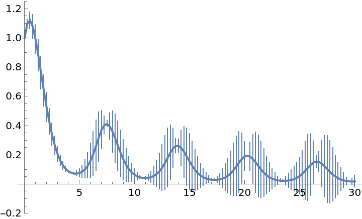 |
Plot the function and its derivative with 2D error bars:
| In[3]:= |
| Out[3]= | 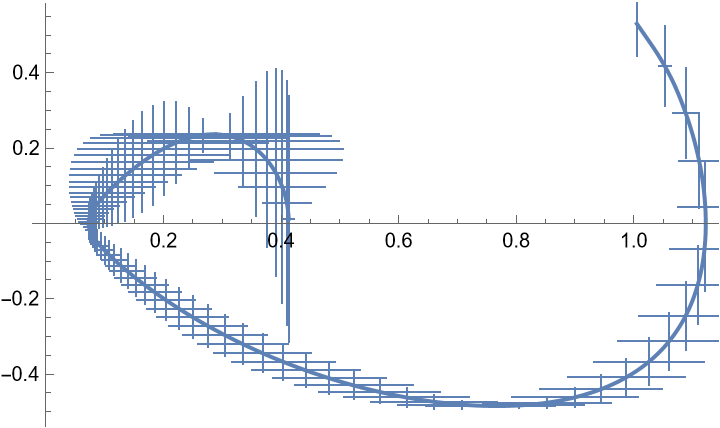 |
Compute the derivatives of the "Value" and "Uncertainty" of the Around quantities independently and re-bundle them inside of Around:
| In[4]:= |
| Out[4]= |
System of ordinary differential equations with uncertainty in the parameters:
| In[5]:= | ![s = ResourceFunction["NDSolveAround"][{
x'[t] == -y[t] - Around[1, 0.05]*x[t]^2,
y'[t] == Around[2, 0.04]* x[t] - y[t]^3,
x[0] == 1,
y[0] == 1
}, {x, y}, {t, 20}];](https://www.wolframcloud.com/obj/resourcesystem/images/cb4/cb4b3f45-b39a-4f13-9907-7be573a95213/2d68d8fdb1310a55.png) |
| In[6]:= |
| Out[6]= | 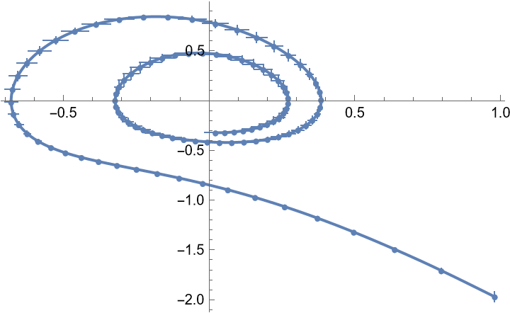 |
Solve the heat equation in one dimension with uncertainty in the thermal diffusivity:
| In[7]:= | ![sol = ResourceFunction["NDSolveAround"][{
D[u[t, x], t] == Around[1, 1] D[u[t, x], x, x],
u[0, x] == 0,
u[t, 0] == Sin[t],
u[t, 5] == 0
}, {u}, {t, 0, 10}, {x, 0, 5}];](https://www.wolframcloud.com/obj/resourcesystem/images/cb4/cb4b3f45-b39a-4f13-9907-7be573a95213/0f80870cd361b3ff.png) |
| In[8]:= | ![points = Flatten[Table[{t, x, sol[[1]][t, x]}, {t, 0, 10, 0.1}, {x, 0, 5, 0.1}], 1];
lowerbound = points /. a_Around :> a["Interval"][[1, 1]];
upperbound = points /. a_Around :> a["Interval"][[1, 2]];
ListPlot3D[{points, lowerbound, upperbound}, PlotRange -> All, PlotStyle -> {Automatic, Directive[ColorData[97, 4]], Directive[ColorData[97, 1]]}]](https://www.wolframcloud.com/obj/resourcesystem/images/cb4/cb4b3f45-b39a-4f13-9907-7be573a95213/1f5976255d4b9960.png) |
| Out[11]= | 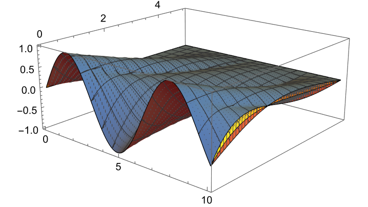 |
Use higher order series expansions to propagate the gaussian error:
| In[12]:= | ![sols = Table[ResourceFunction["NDSolveAround"][{\!\(
\*SubscriptBox[\(\[PartialD]\), \(t, t\)]\(\[Theta][t]\)\) == Around[-9.8, 1]*\[Theta][t], \[Theta][0] == \[Pi]/
4, \[Theta]'[0] == 0
}, {\[Theta]}, {t, 0, 10}, "AroundReplaceOrder" -> n, "NDOptions" -> {Terms -> 6, Scale -> 2}], {n, 1, 4}];
GraphicsGrid@
Partition[
Table[ListLinePlot[Table[{t, sols[[n]][[1]][t]}, {t, 0, 10, 0.1}], PlotLabel -> "\"AroundReplaceOrder\" -> " <> ToString[n], PlotRange -> All], {n, 1, Length[sols]}], 2]](https://www.wolframcloud.com/obj/resourcesystem/images/cb4/cb4b3f45-b39a-4f13-9907-7be573a95213/228e4ec67ea98744.png) |
| Out[13]= | 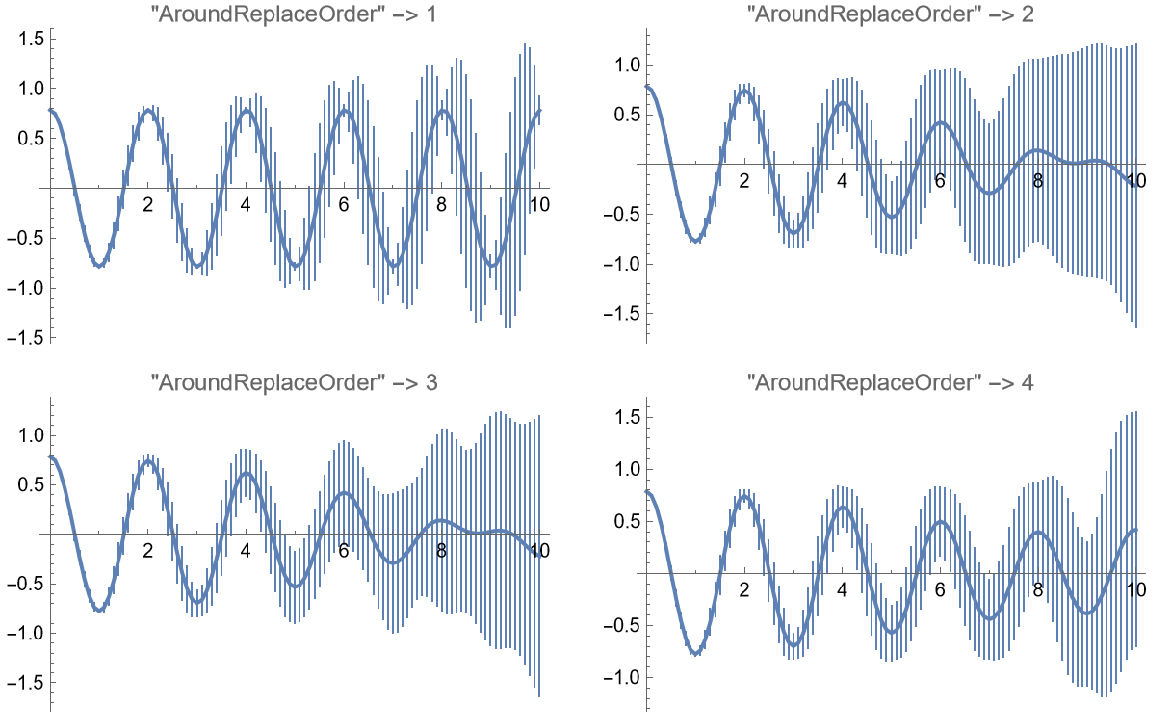 |
Compare the results to an analytical solution using AroundReplace:
| In[16]:= | ![L = Around[1, 0.1];
sol = L = Quantity[Around[1, 0.1], "Meters"];
g = Quantity[1, "StandardAccelerationOfGravity"];
sol = ResourceFunction["NDSolveAround"][Evaluate@{
\!\(
\*SubscriptBox[\(\[PartialD]\), \(t, t\)]\(\[Theta][t]\)\) == Quantity[1, "Seconds"]^2 (-g)/L \[Theta][t],
\[Theta][0] == \[Pi]/4,
\[Theta]'[0] == 0
}, {\[Theta]}, {t, 0, 10}, "AroundReplaceOrder" -> 4, "NDOptions" -> {Scale -> 2, Terms -> 6}];
ListLinePlot[{
Table[{t, AroundReplace[
1/4 \[Pi] Cos[Quantity[1, "Seconds"] (Sqrt[g] t)/Sqrt[l]], {l -> L}, 4]}, {t, 0, 10, 0.1}],
Table[{t, sol[[1]][t]}, {t, 0, 10, 10/100}]
}, PlotStyle -> {Automatic}, PlotLegends -> {"AroundReplace", "NDSolveAround"}]](https://www.wolframcloud.com/obj/resourcesystem/images/cb4/cb4b3f45-b39a-4f13-9907-7be573a95213/56d42da46ed6ba9b.png) |
| Out[20]= | 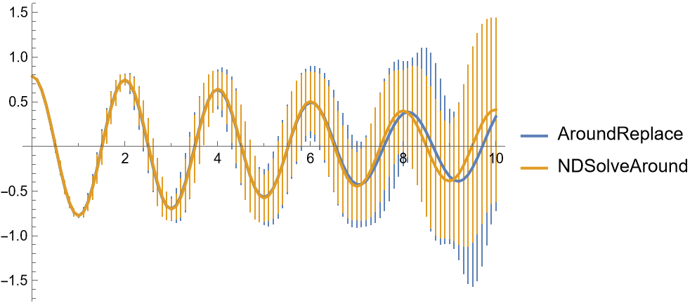 |
Perform a Monte Carlo Simulation and compare the results to the values predicted using NDSolveAround:
| In[21]:= | ![SolveSystem[a_?NumericQ] := NDSolveValue[Evaluate@{\!\(
\*SubscriptBox[\(\[PartialD]\), \(t, t\)]\(\[Theta][t]\)\) == a \[Theta][t], \[Theta][0] == \[Pi]/4, \[Theta]'[0] == 0}, {\[Theta]}, {t, 0, 10}];
Solutions = SolveSystem /@ RandomVariate[NormalDistribution[-9.8, 1], 1000];
MCPoints = Table[{t, Around[Mean[#], StandardDeviation[#]] &@(#[t] & /@ Solutions[[1 ;; -1, 1]])}, {t, 0, 10, 0.1}];
sol = ResourceFunction["NDSolveAround"][Evaluate@{\!\(
\*SubscriptBox[\(\[PartialD]\), \(t, t\)]\(\[Theta][t]\)\) == Around[-9.8, 1]* \[Theta][t], \[Theta][0] == \[Pi]/
4, \[Theta]'[0] == 0}, {\[Theta]}, {t, 0, 10}, "AroundReplaceOrder" -> 4, "NDOptions" -> {Scale -> 2, Terms -> 6}];
Points = Table[{t, sol[[1]][t]}, {t, 0, 10, 0.1}];
ListLinePlot[{Points, MCPoints}, PlotLegends -> {"NDSolveAround", "Monte Carlo Simulation"}]](https://www.wolframcloud.com/obj/resourcesystem/images/cb4/cb4b3f45-b39a-4f13-9907-7be573a95213/6c845a540758a2e5.png) |
| Out[26]= | 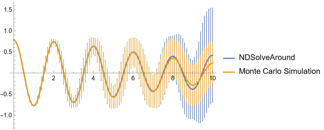 |
In contrast to NDSolve or NDSolveValue, NDSolveAround requires the function specifications to be given in a list:
| In[27]:= |
| In[28]:= |
| Out[28]= |
| In[29]:= |
| In[30]:= |
| Out[30]= |
If the ND Scale and Terms options are not sufficient there may be significant error in the predicted values:
| In[31]:= | ![SolveSystem[a_?NumericQ] := NDSolveValue[Evaluate@{\!\(
\*SubscriptBox[\(\[PartialD]\), \(t, t\)]\(\[Theta][t]\)\) == a \[Theta][t], \[Theta][0] == \[Pi]/4, \[Theta]'[0] == 0}, {\[Theta]}, {t, 0, 10}];
Solutions = SolveSystem /@ RandomVariate[NormalDistribution[-9.8, 1], 1000];
MCPoints = Table[{t, Around[Mean[#], StandardDeviation[#]] &@(#[t] & /@ Solutions[[1 ;; -1, 1]])}, {t, 0, 10, 0.1}];
sol = ResourceFunction["NDSolveAround"][Evaluate@{\!\(
\*SubscriptBox[\(\[PartialD]\), \(t, t\)]\(\[Theta][t]\)\) == Around[-9.8, 1]* \[Theta][t], \[Theta][0] == \[Pi]/
4, \[Theta]'[0] == 0}, {\[Theta]}, {t, 0, 10}, "AroundReplaceOrder" -> 4, "NDOptions" -> {Scale -> 1, Terms -> 11}];
Points = Table[{t, sol[[1]][t]}, {t, 0, 10, 0.1}];
ListLinePlot[{Points, MCPoints}, PlotLegends -> {"NDSolveAround", "Monte Carlo Simulation"}]](https://www.wolframcloud.com/obj/resourcesystem/images/cb4/cb4b3f45-b39a-4f13-9907-7be573a95213/61634d1400474398.png) |
| Out[36]= | 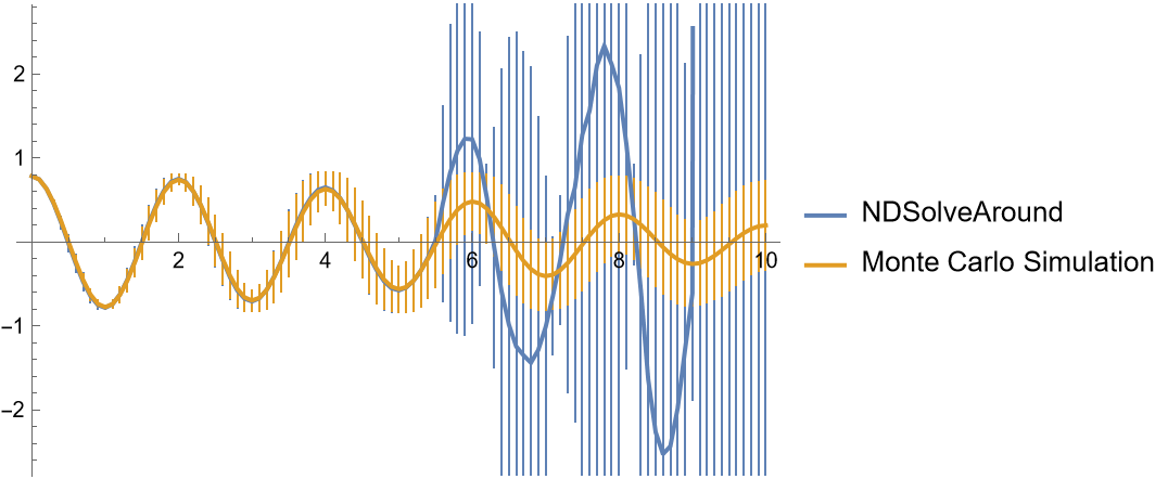 |
Wolfram Language 13.0 (December 2021) or above
This work is licensed under a Creative Commons Attribution 4.0 International License