Wolfram Function Repository
Instant-use add-on functions for the Wolfram Language
Function Repository Resource:
Fit multiple datasets with multiple expressions that share parameters
ResourceFunction["MultiNonlinearModelFit"][{dat1,dat2,…},{form1,form2,…},{β1,…},{x1,…}] is a generalized form of NonlinearModelFit where each dataset dati is fitted with expression formi. The expressions are allowed to share parameter values βi with each other. | |
ResourceFunction["MultiNonlinearModelFit"][{dat1,dat2, …}, <|"Expressions"→{form1,form2,…}, "Constraints"→cons |>, {β1,…},{x1,…}] fits the model subject to parameter constraints cons. |
 (\[FormalN]) to switch between the different expressions formi. This symbol should therefore be avoided by the user when using ResourceFunction["MultiNonlinearModelFit"]. This symbol can be changed with the "DatasetIndexSymbol" option.
Fit some random data to simple linear models with a shared slope parameter:
| In[1]:= | ![data = RandomVariate[BinormalDistribution[0.7], {2, 100}];
data[[1, All, 2]] += 1.;
data[[2, All, 2]] += -1.;
fit = ResourceFunction["MultiNonlinearModelFit"][
data,
{a x + b1, a x + b2}, {a, b1, b2}, {x}
]](https://www.wolframcloud.com/obj/resourcesystem/images/15d/15da9ad9-75bb-46b2-b337-0cfe0fb220f9/31a27ab25902c243.png) |
| Out[4]= |  |
| In[5]:= | ![Show[
ListPlot[data],
Plot[{fit[1, x], fit[2, x]}, {x, -5, 5}]
]](https://www.wolframcloud.com/obj/resourcesystem/images/15d/15da9ad9-75bb-46b2-b337-0cfe0fb220f9/2a8c407edf6c09f8.png) |
| Out[5]= | 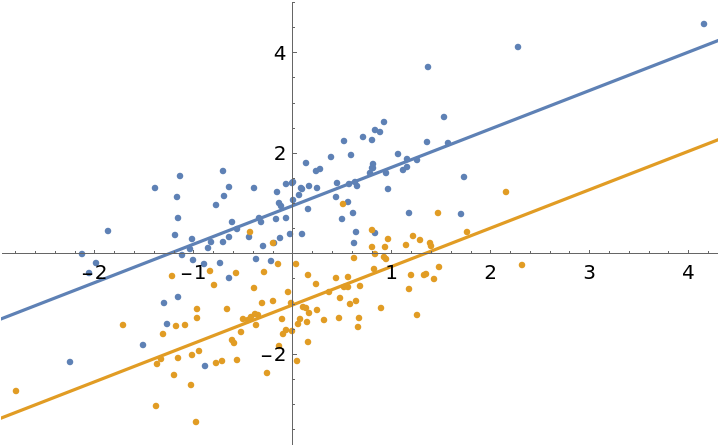 |
Fit the same model with parameter constraints to allow for a small difference between the slopes of the lines (this works best by using a quadratic form for the difference between the slope parameters, since (a1-a2)2is differentiable whereas Abs[a1–a2] is not):
| In[6]:= | ![fit = ResourceFunction["MultiNonlinearModelFit"][
data,
<|
"Expressions" -> {a1 x + b1, a2 x + b2},
"Constraints" -> (a1 - a2)^2 < 0.1^2 && b1 > 0 && b2 < 0 |>,
{a1, a2, b1, b2},
{x}
]](https://www.wolframcloud.com/obj/resourcesystem/images/15d/15da9ad9-75bb-46b2-b337-0cfe0fb220f9/61e2dffac73f0a1e.png) |
| Out[6]= |  |
| In[7]:= | ![Show[
ListPlot[data],
Plot[{fit[1, x], fit[2, x]}, {x, -5, 5}]
]](https://www.wolframcloud.com/obj/resourcesystem/images/15d/15da9ad9-75bb-46b2-b337-0cfe0fb220f9/42e21239c16b62f5.png) |
| Out[7]= | 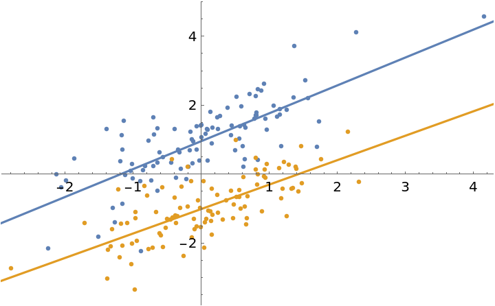 |
It is possible to define a fitting function that evaluates to a list of values equal to the number of datasets when provided with numerical parameters:

The fit function does not evaluate symbolically, only numerically:
| In[8]:= | ![fitfun[{a, b1, b2}, x]](https://www.wolframcloud.com/obj/resourcesystem/images/15d/15da9ad9-75bb-46b2-b337-0cfe0fb220f9/1d36e05bde95a34e.png) |
| Out[8]= |  |
| In[9]:= | ![fitfun[{1, -1, 1}, 2]](https://www.wolframcloud.com/obj/resourcesystem/images/15d/15da9ad9-75bb-46b2-b337-0cfe0fb220f9/2094c973202165ee.png) |
| Out[9]= |  |
Use this function to fit with:
| In[10]:= | ![fit = ResourceFunction["MultiNonlinearModelFit"][
data,
fitfun[{a, b1, b2}, x],
{a, b1, b2},
{x}
]](https://www.wolframcloud.com/obj/resourcesystem/images/15d/15da9ad9-75bb-46b2-b337-0cfe0fb220f9/48f513d9ae6fe44d.png) |
| Out[10]= |  |
| In[11]:= | ![Show[
ListPlot[data],
Plot[{fit[1, x], fit[2, x]}, {x, -5, 5}]
]](https://www.wolframcloud.com/obj/resourcesystem/images/15d/15da9ad9-75bb-46b2-b337-0cfe0fb220f9/00f469b4997487d5.png) |
| Out[11]= | 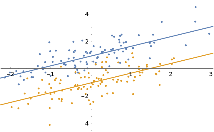 |
Fit two Gaussian peaks with a shared location parameter:
| In[12]:= | ![xvals = Range[-5, 5, 0.1];
gauss[x_] := Evaluate@PDF[NormalDistribution[], x];
With[{amp1 = 1.2, amp2 = 0.5, width1 = 1, width2 = 2, sharedOffset = 0.5, eps = 0.05},
dat1 = Table[{x, amp1 gauss[(x - sharedOffset)/width1] + eps RandomVariate[NormalDistribution[]]}, {x, xvals}];
dat2 = Table[{x, amp2 gauss[(x - sharedOffset)/width2] + eps RandomVariate[NormalDistribution[]]}, {x, xvals}]
];
plot = ListPlot[{dat1, dat2}]](https://www.wolframcloud.com/obj/resourcesystem/images/15d/15da9ad9-75bb-46b2-b337-0cfe0fb220f9/510c701533c5cab5.png) |
| Out[13]= | 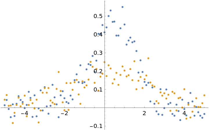 |
Fit with the models that were used to generate the data:
| In[14]:= | ![fit = ResourceFunction["MultiNonlinearModelFit"][
{dat1, dat2},
{
amp1 gauss[(x - sharedOffset)/width1],
amp2 gauss[(x - sharedOffset)/width2]
},
{amp1, amp2, width1, width2, sharedOffset},
{x}
]](https://www.wolframcloud.com/obj/resourcesystem/images/15d/15da9ad9-75bb-46b2-b337-0cfe0fb220f9/30ffda093f505e2b.png) |
| Out[14]= |  |
| In[15]:= | ![fit["BestFitParameters"]](https://www.wolframcloud.com/obj/resourcesystem/images/15d/15da9ad9-75bb-46b2-b337-0cfe0fb220f9/13c26acaa837ddb2.png) |
| Out[15]= |  |
Extract the fits as a list of expressions:
| In[16]:= | ![fits = fit[#, x] & /@ {1, 2}](https://www.wolframcloud.com/obj/resourcesystem/images/15d/15da9ad9-75bb-46b2-b337-0cfe0fb220f9/25bb9a2d4feccdb8.png) |
| Out[16]= |  |
Compare the fits to the data:
| In[17]:= | ![Show[
plot,
Plot[fits, {x, -5, 5}]
]](https://www.wolframcloud.com/obj/resourcesystem/images/15d/15da9ad9-75bb-46b2-b337-0cfe0fb220f9/080f679192c49df0.png) |
| Out[17]= | 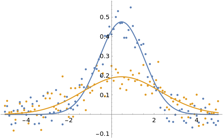 |
The Weights option can be specified in a number of ways. First generate datasets with an unequal number of points and offset them slightly:
| In[18]:= | ![gauss[x_] := Evaluate@PDF[NormalDistribution[], x];
With[{amp1 = 1.2, amp2 = 0.5, width1 = 1, width2 = 2, sharedOffset = 0.5, eps = 0.025},
dat1 = Table[
{x, amp1 gauss[(x - sharedOffset)/width1] + eps RandomVariate[NormalDistribution[]]},
{x, -5, 5, 0.1}
];
dat2 = Table[
{x, amp2 gauss[(x - sharedOffset + 1)/width2] + eps RandomVariate[NormalDistribution[]]},
{x, -5, 5, 0.2}
]
];
fitfuns = {
amp1 gauss[(x - sharedOffset)/width1],
amp2 gauss[(x - sharedOffset)/width2]
};
fitParams = {amp1, amp2, width1, width2, sharedOffset};
variables = {x};
plot = ListPlot[{dat1, dat2}]](https://www.wolframcloud.com/obj/resourcesystem/images/15d/15da9ad9-75bb-46b2-b337-0cfe0fb220f9/474de872d6a223e5.png) |
| Out[19]= | 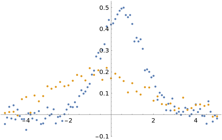 |
Fit the data normally. In this case, each individual data point has equal weights in the fit, so the first dataset gets more weight overall since it has more points:
| In[20]:= | ![fit1 = ResourceFunction["MultiNonlinearModelFit"][
{dat1, dat2},
fitfuns, fitParams, variables
];
fit1["BestFitParameters"]](https://www.wolframcloud.com/obj/resourcesystem/images/15d/15da9ad9-75bb-46b2-b337-0cfe0fb220f9/16b0c62543a9ca82.png) |
| Out[21]= |  |
| In[22]:= | ![Show[plot, Plot[{fit1[1, x], fit1[2, x]}, {x, -5, 5}]]](https://www.wolframcloud.com/obj/resourcesystem/images/15d/15da9ad9-75bb-46b2-b337-0cfe0fb220f9/510c7aa41b5701a2.png) |
| Out[22]= | 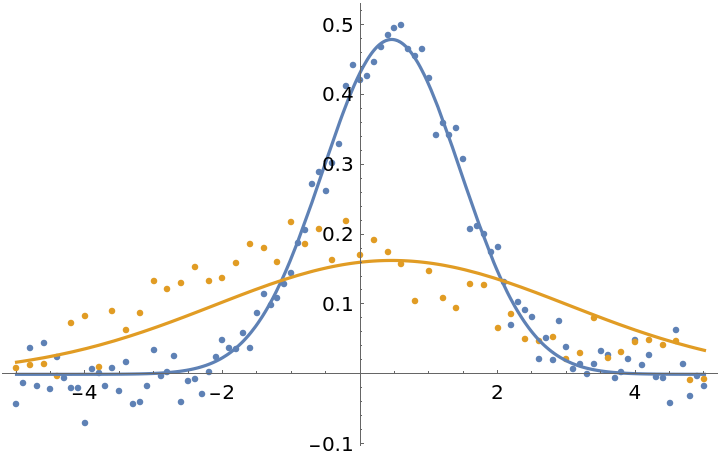 |
Assign more weight to the second dataset:
| In[23]:= | ![fit2 = ResourceFunction["MultiNonlinearModelFit"][
{dat1, dat2},
fitfuns, fitParams, variables,
Weights -> {1, 20}
];
fit2["BestFitParameters"]](https://www.wolframcloud.com/obj/resourcesystem/images/15d/15da9ad9-75bb-46b2-b337-0cfe0fb220f9/3d1d77cb250e5d78.png) |
| Out[24]= |  |
| In[25]:= | ![Show[plot, Plot[{fit2[1, x], fit2[2, x]}, {x, -5, 5}]]](https://www.wolframcloud.com/obj/resourcesystem/images/15d/15da9ad9-75bb-46b2-b337-0cfe0fb220f9/6419f1670f159591.png) |
| Out[25]= | 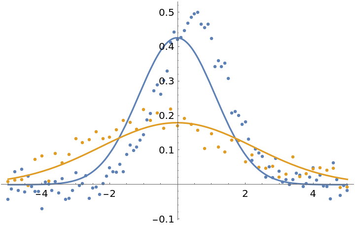 |
Assign weights inversely proportional to the number of points in the dataset. This asserts that each dataset is equally important:
| In[26]:= | ![fit3 = ResourceFunction["MultiNonlinearModelFit"][
{dat1, dat2},
fitfuns, fitParams, variables,
Weights -> "InverseLengthWeights"
];
fit3["BestFitParameters"]](https://www.wolframcloud.com/obj/resourcesystem/images/15d/15da9ad9-75bb-46b2-b337-0cfe0fb220f9/6132b236a57024e8.png) |
| Out[27]= |  |
| In[28]:= | ![Show[plot, Plot[{fit3[1, x], fit3[2, x]}, {x, -5, 5}]]](https://www.wolframcloud.com/obj/resourcesystem/images/15d/15da9ad9-75bb-46b2-b337-0cfe0fb220f9/5cb85b811925b785.png) |
| Out[28]= | 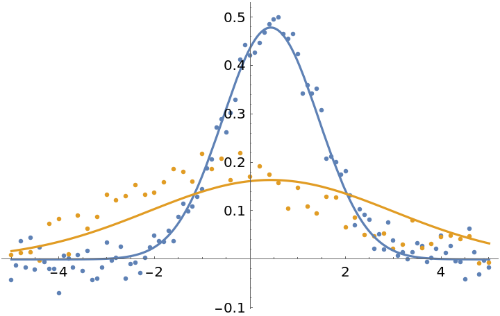 |
To assign weights for each individual data point, you can pass a list of vectors matching the input data:
| In[29]:= | ![fit4 = ResourceFunction["MultiNonlinearModelFit"][
{dat1, dat2},
fitfuns, fitParams, variables,
Weights -> {
RandomReal[{0, 1}, Length[dat1]],
RandomReal[{0, 1}, Length[dat2]]
}
];
fit4["BestFitParameters"]](https://www.wolframcloud.com/obj/resourcesystem/images/15d/15da9ad9-75bb-46b2-b337-0cfe0fb220f9/70f3b4dc1c314777.png) |
| Out[30]= |  |
| In[31]:= | ![Show[plot, Plot[{fit4[1, x], fit4[2, x]}, {x, -5, 5}]]](https://www.wolframcloud.com/obj/resourcesystem/images/15d/15da9ad9-75bb-46b2-b337-0cfe0fb220f9/2124fdb07d957ac4.png) |
| Out[31]= | 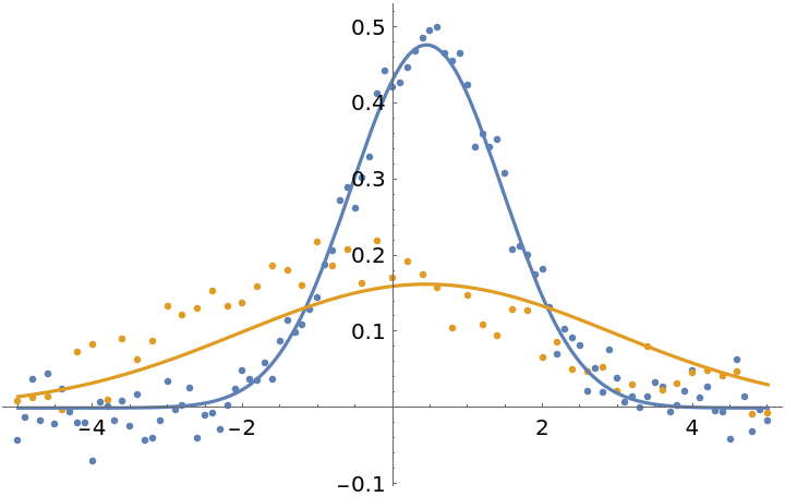 |
Use a different symbol to index the datasets:
| In[32]:= | ![fit = ResourceFunction["MultiNonlinearModelFit"][
RandomVariate[BinormalDistribution[0.7], {2, 100}],
{a x + b1, a x + b2}, {a, b1, b2}, {x}, "DatasetIndexSymbol" -> mySymbol];
Normal[fit]](https://www.wolframcloud.com/obj/resourcesystem/images/15d/15da9ad9-75bb-46b2-b337-0cfe0fb220f9/6d1d7f52862226c1.png) |
| Out[33]= |  |
| In[34]:= | ![Table[Normal[fit], {mySymbol, {1, 2}}]](https://www.wolframcloud.com/obj/resourcesystem/images/15d/15da9ad9-75bb-46b2-b337-0cfe0fb220f9/2529aca70f17f8eb.png) |
| Out[34]= |  |
This work is licensed under a Creative Commons Attribution 4.0 International License