Wolfram Function Repository
Instant-use add-on functions for the Wolfram Language
Function Repository Resource:
Find the numerical derivative of a list of values or pairs of values
ResourceFunction["ListD"][data] finds the derivative of a list of data. | |
ResourceFunction["ListD"][data,type] finds the derivative of a list of data using the method type. |
| "WindowSize" | 1 | the number of extra points to use to find a linear fit |
Find the derivative of data sampled from a function:
| In[1]:= |
| Out[1]= |
| In[2]:= |
| Out[2]= |  |
| In[3]:= |
| Out[3]= | 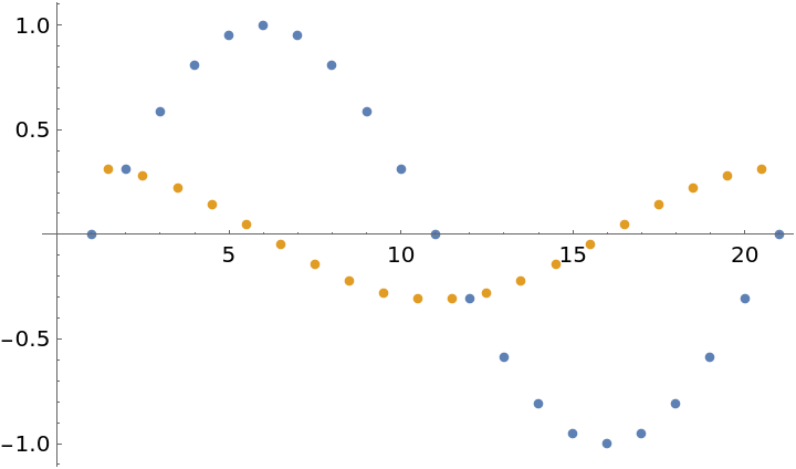 |
Find the derivative of {x,y} data sampled from a function:
| In[4]:= |
| Out[4]= |  |
| In[5]:= |
| Out[5]= |  |
| In[6]:= |
| Out[6]= | 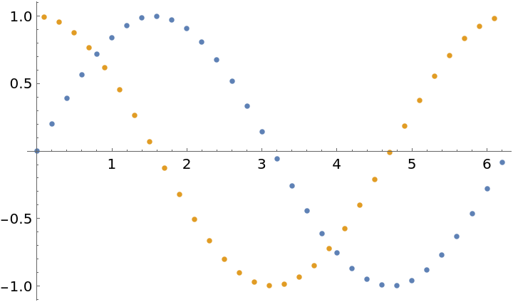 |
The default method, "Center" generates new points between each of the original x-values using values from both sides to approximate the derivative:
| In[7]:= |
| Out[7]= |
The method, "Forward" generates new points at each of the original x-values using the next values to determine the derivative:
| In[8]:= |
| Out[8]= |
The method, "Backward" generates new points at each of the original x-values using the previous values to determine the derivative:
| In[9]:= |
| Out[9]= |
The method, "Fourier" is appropriate for larger sets of oscillatory data:
| In[10]:= |
| In[11]:= |
| Out[11]= | 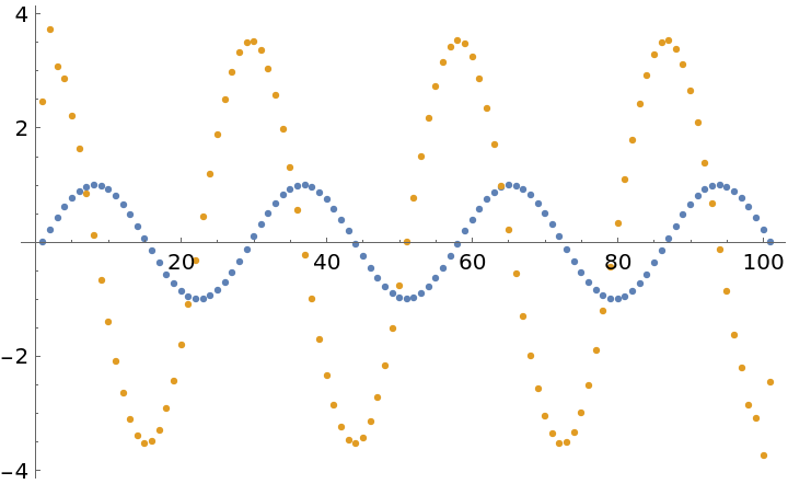 |
A small amount of noise in data can create significant errors in ListD:
| In[12]:= | ![data3 = Table[{x, Sin[x] + RandomReal[{-0.1, 0.1}]}, {x, 0., 2 Pi, 0.1}];
ListPlot[{data3, ResourceFunction["ListD"][data3]}]](https://www.wolframcloud.com/obj/resourcesystem/images/081/081a7167-088d-4a88-8790-6fba88931b10/30f08dcda82938b5.png) |
| Out[13]= | 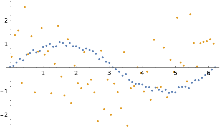 |
By increasing the "WindowSize" the derivative is established by from the best local fit to the points:
| In[14]:= |
| Out[14]= | 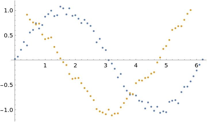 |
Smoothing the data first to remove noise has a similar effect but often produces less smooth results for the same amount of smoothing:
| In[15]:= |
| Out[15]= | 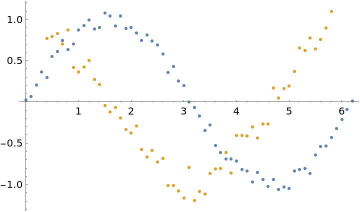 |
The "Fourier" method is only supported for regularly sampled data:
| In[16]:= |
| Out[16]= |
This work is licensed under a Creative Commons Attribution 4.0 International License