Wolfram Function Repository
Instant-use add-on functions for the Wolfram Language
Function Repository Resource:
Compute the GCD and successive quotients for a pair of Laurent polynomials
ResourceFunction["LaurentExtendedGCD"][p1,p2,x] computes the extended GCD of the Laurent polynomials p1 and p2 in x. |
Compute a quotient sequence and GCD for two polynomials:
| In[1]:= |
| Out[1]= |
Create a pair of random Laurent polynomials of degree 10:
| In[2]:= | ![SeedRandom[1234];
n = 11;
mid = Quotient[n, 2];
lpoly1 = N@RandomInteger[100, n] . z^Range[-mid, mid];
lpoly2 = N@RandomInteger[100, n] . z^Range[-mid, mid];
{lpoly1, lpoly2}](https://www.wolframcloud.com/obj/resourcesystem/images/395/395e8142-f326-4520-9a17-0974f57f22b2/019697602154fe78.png) |
| Out[7]= |  |
Compute a quotient sequence and GCD:
| In[8]:= |
| Out[8]= |  |
Create two exact Laurent polynomials:
| In[9]:= | ![SeedRandom[1234];
n = 5;
mid = Quotient[n, 2];
lpoly1 = RandomInteger[100, n] . z^Range[-mid, mid];
lpoly2 = RandomInteger[100, n] . z^Range[-mid, mid];
{lpoly1, lpoly2}](https://www.wolframcloud.com/obj/resourcesystem/images/395/395e8142-f326-4520-9a17-0974f57f22b2/68325328262918ec.png) |
| Out[10]= |
Compute a quotient sequence and GCD:
| In[11]:= |
| Out[11]= |  |
LaurentExtendedGCD can return a nontrivial GCD:
| In[12]:= | ![SeedRandom[1234];
n = 5;
mid = Quotient[n, 2];
lpoly1a = RandomInteger[100, n] . z^Range[-mid, mid];
lpoly2a = RandomInteger[100, n] . z^Range[-mid, mid];
lpoly3 = RandomInteger[100, n] . z^Range[-mid, mid];
{lpoly1, lpoly2} = Expand[{lpoly1a, lpoly2a} lpoly3]](https://www.wolframcloud.com/obj/resourcesystem/images/395/395e8142-f326-4520-9a17-0974f57f22b2/504d6278b2d0c330.png) |
| Out[13]= |  |
Compute a quotient sequence and GCD:
| In[14]:= |
| Out[14]= |  |
LaurentExtendedGCD works with approximate numeric coefficients and gives an equivalent result:
| In[15]:= |
| Out[15]= |  |
Compare the difference numerically:
| In[16]:= |
| Out[16]= |
Form the Laurent pair corresponding to the Daubechies 6 (or db3) wavelet filter coefficients:
| In[17]:= | ![coeffsD6 = Sqrt[2] Last /@ WaveletFilterCoefficients[DaubechiesWavelet[3], "PrimalLowpass", WorkingPrecision -> \[Infinity]];
{evenD6, oddD6} = N@Transpose[Partition[coeffsD6, 2]] . z^(
2 - Range[Length[coeffsD6]/2])](https://www.wolframcloud.com/obj/resourcesystem/images/395/395e8142-f326-4520-9a17-0974f57f22b2/56f5c0571ac1fe2a.png) |
| Out[18]= |
Compute the GCD and quotients:
| In[19]:= |
| Out[19]= |
A set of quotients and remainder can also be obtained using WaveletFilterCoefficients with "LiftingFilter" and "LiftingLaurentForm":
| In[20]:= |
| Out[21]= |
Obtain the Daubechies 4 (D4, also called db2) wavelet coefficients:
| In[22]:= | ![coeffsD4 = Sqrt[2] Last /@ WaveletFilterCoefficients[DaubechiesWavelet[2], "PrimalLowpass", WorkingPrecision -> \[Infinity]]](https://www.wolframcloud.com/obj/resourcesystem/images/395/395e8142-f326-4520-9a17-0974f57f22b2/2b355098172e55a1.png) |
| Out[22]= |
Create two corresponding Laurent polynomials:
| In[23]:= |
| Out[23]= |
Compute the Laurent GCD and list of quotients:
| In[24]:= |
| Out[24]= |
Create a list of 2×2 matrices that represent the operation of reducing a pair of Laurent polynomials by their quotient:
| In[25]:= |
| Out[26]= |
Take their product:
| In[27]:= |
| Out[27]= |
Applying this product to the vector comprised of the GCD and 0 recovers the original pair of Laurent polynomials:
| In[28]:= |
| Out[28]= |
Invert the reducing matrices:
| In[29]:= |
| Out[30]= |
Form the reverse-product of these inverses:
| In[31]:= |
| Out[31]= |
Check that this is in fact the inverse:
| In[32]:= |
| Out[32]= |
This inverse product matrix provides the Bezout multipliers (top row) and syzygy (bottom row), as can be seen by its action on the input pair:
| In[33]:= |
| Out[33]= |
Create the quadrature mirror filter from the D4 coefficients:
| In[34]:= |
| Out[34]= |
A certain upper triangular matrix is needed to recover these Laurent polynomials:
| In[35]:= |
| Out[35]= |
Form the augmented set of 2×2 matrices required to create the wavelet polyphase matrix:
| In[36]:= | ![smat = {{1, sval}, {0, 1}};
scalingmat = {{gd4, 0}, {0, 1/gd4}};
allmats = Join[qmats, {smat, scalingmat}]](https://www.wolframcloud.com/obj/resourcesystem/images/395/395e8142-f326-4520-9a17-0974f57f22b2/78fb8474b9e2732c.png) |
| Out[37]= |  |
Compute the polyphase matrix:
| In[38]:= |
| Out[38]= |
Show that the second column is indeed the quadrature mirror filter:
| In[39]:= |
| Out[39]= |
The same matrix can be obtained from WaveletFilterCoefficients:
| In[40]:= | ![lf = WaveletFilterCoefficients[DaubechiesWavelet[2], "BestLiftingFilter"];
lf[{"PolyphaseMatrix", z}]](https://www.wolframcloud.com/obj/resourcesystem/images/395/395e8142-f326-4520-9a17-0974f57f22b2/0ae6bdcb9491168b.png) |
| Out[41]= |
Create a function to recover the discrete wavelet transform (DWT) from these 2×2 matrix factors. For this, powers of the Laurent variable z become shifts with positive exponents being leftward, and indices are modulo the length of the sequence (that is, using periodic wrapping):
| In[42]:= | ![extractpart[v_, i_, m_] := v[[Mod[i, m, 1]]];
operate[a_Real, v_, i_, n_] := a*extractpart[v, i, n]
operate[a_Real*z^e_., v_, i_, n_] := a*extractpart[v, i - e, n]
operate[aa_Plus, v_, i_, n_] := Map[operate[#, v, i, n] &, aa]
operateMat[mat_?MatrixQ, vecs_?MatrixQ, n_] := Table[{operate[mat[[1, 1]], vecs[[1]], j, n] + operate[mat[[1, 2]], vecs[[2]], j, n], operate[mat[[2, 1]], vecs[[1]], j, n] + operate[mat[[2, 2]], vecs[[2]], j, n]}, {j, Length[vecs[[1]]]}]](https://www.wolframcloud.com/obj/resourcesystem/images/395/395e8142-f326-4520-9a17-0974f57f22b2/27453a0b242436d0.png) |
Work with {1,2,…,16} split into odds and evens (the so-called "Lazy Wavelet Transform"):
| In[43]:= | ![vec16 = Range[16];
{odds16, evens16} = {vec16[[1 ;; -1 ;; 2]], vec16[[2 ;; -1 ;; 2]]};
oddsevens = {odds16, evens16};
nmats = N[Collect[allmats, z]];](https://www.wolframcloud.com/obj/resourcesystem/images/395/395e8142-f326-4520-9a17-0974f57f22b2/109a5da633be76a9.png) |
Compute the DWT:
| In[44]:= |
| Out[44]= |
Compare to the forward lift from the LiftingFilterData for the D2 wavelet:
| In[45]:= |
| Out[45]= |
Get the same result directly from LiftingWaveletTransform:
| In[46]:= |
| Out[46]= |
Invert the process to recover the original values, using Riffle at the end to undo the Lazy Wavelet Transform:
| In[47]:= |
| Out[48]= |
This is equivalent to using InverseWaveletTransform on the DiscreteWaveletData object:
| In[49]:= |
| Out[49]= |
The conventional way to use the quotient matrices and their inverses to form a lifting filter actually makes them alternating upper and lower triangular. For simplicity of exposition, this step was omitted.
Create the even and odd Laurent polynomials that arise from the Daubechies10 wavelet coefficients:
| In[50]:= | ![coeffsD10 = Sqrt[2] Last /@ WaveletFilterCoefficients[DaubechiesWavelet[5], "PrimalLowpass", WorkingPrecision -> 100];
hpoly = coeffsD10*(1/z)^(Range[Length[coeffsD10]] - 1);
N[{evenpoly, oddpoly} = Expand[z*Plus @@@ Transpose[Partition[hpoly, 2]] /. z^n_ :> z^Ceiling[n/2]]]](https://www.wolframcloud.com/obj/resourcesystem/images/395/395e8142-f326-4520-9a17-0974f57f22b2/2d7f97df41d2df66.png) |
| Out[52]= |  |
Compute an extended GCD with quotients coefficients that are reasonably close in magnitude to unity:
| In[53]:= |
| Out[53]= |
Another good set of quotients for the D10 Laurent pair is given in the reference by Maslen and Abbott; the latter happens to be the one provided by WaveletFilterCoefficients:
| In[54]:= |
| Out[55]= |  |
Create the quotient matrices and the scaling value (a factor of z2 is required for this particular factorization):
| In[56]:= | ![makeQMatrix[lpoly_] := {{lpoly, 1}, {1, 0}}
qmats = Map[makeQMatrix, quotsD10];
gvec = {oddpoly, -evenpoly} /. z -> 1/z;
qprod = Expand[Apply[Dot, qmats]];
vec = Expand[
qprod . {{gcdD10, 0}, {0, 1/gcdD10}} . {{1, s z^2}, {0, 1}}[[All, 2]] - gvec];
sval = N[s /. First[SolveAlways[vec == 0, z, WorkingPrecision -> 50]]];
smat = {{1, sval}, {0, 1}};
scalingmat = {{gcdD10, 0}, {0, 1/gcdD10}};
allmats = N[Join[qmats, {scalingmat, smat}]]](https://www.wolframcloud.com/obj/resourcesystem/images/395/395e8142-f326-4520-9a17-0974f57f22b2/709f2695b7cbef4f.png) |
| Out[64]= |  |
Set up functions that transform from Laurent polynomials to vector operations:
| In[65]:= | ![extractpart[v_, i_, m_] := v[[Mod[i, m, 1]]];
operate[a_Real, v_, i_, n_] := a*extractpart[v, i, n]
operate[a_Real*z^e_., v_, i_, n_] := a*extractpart[v, i - e, n]
operate[aa_Plus, v_, i_, n_] := Map[operate[#, v, i, n] &, aa]
operateMat[mat_?MatrixQ, vecs_?MatrixQ, n_] := Table[{operate[mat[[1, 1]], vecs[[1]], j, n] + operate[mat[[1, 2]], vecs[[2]], j, n], operate[mat[[2, 1]], vecs[[1]], j, n] + operate[mat[[2, 2]], vecs[[2]], j, n]}, {j, Length[vecs[[1]]]}]](https://www.wolframcloud.com/obj/resourcesystem/images/395/395e8142-f326-4520-9a17-0974f57f22b2/3c260f8da3ed0ed0.png) |
Pad a square image to have a power of 2 dimension, removing the average pixel value from each row:
| In[66]:= | ![img = \!\(\*
GraphicsBox[
TagBox[RasterBox[CompressedData["
1:eJwteod3E9e2t1zovbfQWwgECCWEFiD0EkIJIYRuTAvdptqAwb13S7Jk9V5n
JM2MRlPVuyXL3cZgOuTm3vfe9x98x+TOWvaSl6XZZ5+996+c0dy0W0cuJXM4
nMyh4NeR8w+2ZWScf3R0LPjj2M3Mq5dvXkzfe/PuxcsXM35IG3hb+n9/fteo
bCRhJxwuN8PiDgyxajVqnVZrMWnUCiNk0cslQgG/sf74hn0HDx05euL4kaPH
T1x9kvXofvru6eOXHr5VXC6DHF6GxAm7SasX1xZk3/3jKW7VWgw6ow2zIARu
uwZDjlAg5Pf6XS6f00kQpA22WkxG2KpXKhGXEzdKxY2NgoZ7K9duWr91y5Yd
ey7de1JVX1lc2SDm/blu2vqLD/KqJUYrptcbjDoVt7Tw8fnrdlattSM2xEGR
LGUj7kGEJxqPN8eaAwF/wON00Raz2WQy6wxaLeyJR3y4SSUWNNYWbJr/7bLl
K1fuv/q8tLRI0MSv4kpBsveXL/rlxqPSxiaVVNRUyBXXFdy/fs5AsGqEYB2I
nWEYB4Pm25lAS2ussy3Wkgg0h/1BD4bYLCadGbbCZEv/qxiDaBRNddVlRybP
nTd/4cEbudUVFfymhqqKaqlcq7JJj81feezP+4WF5Q3c4uqa/AfX/6hzUy4b
y5KIhXBghN1hrmNwtr23u/Pli64Xra0xj9tJYCgC6WwE6WA7375qJU1qeROX
W3l2/ISJkw5k5+c/LeBzBU0N/AZek6xRiUJ5P81e9cvl+1m5BSXFT26k/Xrc
gocDeUoXBOMkSZCs3V7lItwdr999ev/+9fvXvQmv20mRX4oC2/Hgyw99MdJi
VEkEDWXnxg4ZvD035/GDEj63qLJOqBBJZFqVTK5Wi64vnL7+1/NXrl/789yx
Pauv0mwbvfcQRWAMbbeRJEMV+Vyh+OvPnz+9//jhzdsXbQF3wO3xh0kMQ+jY
ize9Psqi1UuF3JLfx3NW5z55mJXL4xc/BgUQi6RKE4iv0EgkhT+MXbxp75GD
P+/euGbug4C39/mWfJZmWA/j9gW8zAOPp9nT/vHD20+fP757+7ovFo14PD6f
m6Rd3nCkNcI4DCqdUsDN3T9s1sP7dx+W1nHLnj0prxFIFRq9xawE7SFvqK85
NHrigqXLVy6dN2NMcSzgzLlhp0mG8fnDYZ/Pf9FJhvzx1x/ff3j3/u2b/t7W
ZtBdgZCXplmC9XhYEjPqjXJe3d3Vw4/f/TP7SX1DeX5eYXm9RK9RWZy01QzZ
jIpGXm3ahNQxEyaNHjZomNRPWEQamsLtdjdII9racpKgQqG2zp53/QMRejpa
ogGfN9ziJkgLbEUoEkWMcqVUVHN6+pI79zIfFdVzy0pq6hua1FajlXQ6PYzR
gqFKEa/m1nROchIY6q9gkjBBdtJNkZTHx/hDrdFDEq8vmIi397969eF1d2db
vLk5EAr6HTYYgs0mCwxBeqVKJSnaO/p4aUlucVVVLb+uXqLWIg6HA8csdg+L
wgaVpLGqLGMqJykpmbOOJUiEopwer9Pl8/sDwWjzoedOty8eTrwAV3d3d0ck
EvR6WYfFpDVajAadxqBW6FRS4eM1k29WV9fU1nP5UqlQqtCD27AsYUdREkMQ
SFHPrym+NIKTlMo5EmU8oJY063WHvcFEe2db9MgZ3OMMBiLdr7pjrfHmkC8S
8DB2K2zQm816g16rVIEYEv6NOcvvVQuUPLNRZjAatEqrw+UMRSNgORQGLq24
iV+SuzllyMiUa81eN8AmmmKD7X3dXX3d7fFTWxpDbr/fH4kkWsBnWFcoGvA4
LGbYbNaYrEatXK6Wi8TlZ6Ztzm2USESYVWPCEDtmp31gOa3RQMjH4ihu02m5
NXlpMwdPHPrQ56f9sUgw4E909b9996a/J3Fy23EyEAp7WMIX8ThplvaGAwGX
3WqB9XqLRTswZUqpsOTIlKPVcjNsojxulqV8Ua/TTbO+aCwQikRCjIu1mySN
Zfd+Gj5x6GPK63In2lo6erpevf38r4/v2uNp+1bng2alWQpnSRp3OEhwF9ph
BXlYYKNJp1CpNDJezp6ZV/l6nPX627rbWE/M7/ZSdozxhMEOhJrdbtJu1fPL
c05Pmjgis9XrirS+ePGq/23/539/fv+qo+3Wsa1bIK+HZsHaUbvViBCMx0kS
qNViAbnAeo1WIZPUZKxf9FABmijR1tPd7veFg26WwAna6XIFgz5fs5fAUUNj
4fO0qVNHHm0Oh5qjXW/effr4/q+/P7/uagveO35o7UmWDeCkC0N1fJ64nqYZ
l5NxIAhq0pr0KoVYxC+4vHJ5kdpmd7b093V2JsKRoIsgUIIAydNOhvZSNhui
F5YU/T5x7qxVVCgYCrX0fvj70+fPb1/2gSU9Tj+xa/E9H2jDsJ/U5tWV/JZP
MR43iGGzGrR6o1Ik4pXePfHVwhoFxgR63r2Kt8RCUR8YTowk7SRqQx2Uy2HU
Q7CGW7J+zDd7VhQFQG/6/N39H//6/La3uy0YKr57Yd/G2fdDYCIjjIX79OCq
3dZowM0QKAqbIZ1aKRJUPbu+K3VCqRpxt7zp6wh53bTX50CsKMUyBIZgNOMk
EStuU9Snz1yw88r5Ywjr9XlC4fjr1739Pd3xkK/u+e0Tu5cMT/cH2ZCfMsh4
gnpnc8jvxG1WCIKMCmFjZcn936ZwhmSrjHDoTV97CMyxk7DAJhRDSZqk7Awo
OUVTVnnjia+Wbt62ZVVl2M0yXl880QoitMZcjuq8e+cPfT+ZsxvykixNuTtf
9LVHPU6GdKBGtUYpqK/IeXh2QcqoQb/LZZi/s6cNoKqfslqsJgS2AHAF9SBd
uJXGbWp+wc6Js2d/vfowSrIutz/ojbREfV4/gzWUZ13cs3pGCmd2Fup0kKw/
Gu1oDZAIBulAtYUNVTkZJ78eNWX2rB+EfJiNtjbHw6yfQSDYZEMQG2Z3uxg7
ZjFCKInKBOljZs77dsvWBxYL63Q6vACugrTb6eDlZfyx55spKSkczrpSB2Bf
Ox0NuUkgXqRCmbihPOfPfYu++vaHjeu/fWqQWdlIyOukGFBkkwFCURRDwETR
VhjR2xwOnfSPETMXbj9x7lQZYFIX7h0AAafT66p4fOX4+oWTUzjJKZxxB3JE
ZsgAIBeBDFpRvbCuKOPwhtUbDvzxx9FfNh7U6AxgF0iaIbwOs8YAQTYAr4yT
RglAqA6rpql264g5G28XZZ3cWupBQYlADK/b7bIXZxzfuXLuuGSA/amL16z4
fsfZu88r6hpq6njC2icXd639YfeZtPT0c6eP79+QCWksDgfjIh0kapIbUMzq
IP1+oABAXCcFyequz57+46OmiqsHtiwvoR1AvpEUS4HCPj/zy8Zvpg8H5DJu
xb70tEMb54yYMP+7dZs2b9+6csbQlJnf7ztxLu3chbRTR3ZuLlQoAMAgmAOD
DAod7cAJB2hTykZjJsQmF2aunrnjMff+pTsPH/2+9081heEIBlsJFLp2Ztua
2SM5Kd9ffFxQWFpSWPTkt29Gcv57JQ8es3D9wUN/XLmWfv63A2u2Pigo54vk
eotRa1CrYAS2oTaLWaPWasSCporrG1ccup917mJ+Lb/m1vnDu7JMJNBQYE8N
5/asWjaes/y5xqiRlFfVVVaWF+XePLQc6OSU5OQhw0dMWvrj7jNXLqRfPL53
w6KvN20/evnBs+p6YWM9gB0JXy7l8fkCqaChPOPQ2vW/X7129XFtbW11Q8nV
U9tWb0rP4yp1SrnsyPqVMwefM0AykQ6SV5VX15cXFRaX5l7dOQukkTJi9Oip
K3f9fjbt6G9njx39ecuqeaNHTP/h0IVbd+8/yHmWk/3gQUb243sPM05vmpS6
aNXxR8X1dTyxoKEq//GF4wdXThozb+vZB9k3929aMuY2JFXLjWabSVtfXVdd
VV5ZX1uUk7ljBCdl2MhBI2d8v2//8Yt3n+U3CAS8mkcH5g6dvGr7vt0HDv28
f9dPW39YuXDGxJEpAxt7oFLIr6nlNQl5NUXl986d2PXtuIENHzRk29ppZ6Vl
lXotZDUptDpBZW1VdW2ToK6yJOfYOE7qsNFjJk5bfqaYx5ebYLMCbL28On3x
oLGTxk+aMHbEkKGjRo8ZNQx4jZRBSb9qQPfWVNdWllSVV5Tlp587s3nOkOQB
H/L9/AsqaSPfCMF6pV4k1Ui5dXUCsVjIrS14cnAkJ3XI6EEzM8Rag9lOOew2
MPwapbhqf8o/PTF44rTps2ZPnzRqWMrQ66hKKhWJRPzqirKy4sLS7FuXdi4d
6NekpEW7zLBWCRapk+uASNAqJE1N0iYxr5FbmnfluxROKmdJqVyDETRDIXbU
YjJbAVDyTw/jJHGSR0xbtOSbpUsXzZ05eWKmTQu2QSlXCqoqq6qrqirzstL3
rhzDGZBc32aSqF5vhFGl1m6CbRqhxqyXSVQSsbC29NqmiUmc78V6vR2j3S6X
w27HUDsCYUZZ0zmwC6O+Wvr9xh+3blq1ZunXz1CTwWDQ6bRqcV0tX9jYUFP0
9PKR9ZO+xFihsKGQCbbYDBYW0pnkIhOiBfU3GOT1JTc2zuF8DxocqDUgyQCA
gukD/AeaXi49zBk+ZeHq73fs2XPgpx/XF9qsFgS1mU2QVAwEeD2fX139POPE
xmlftvQnGgFAjdl0KO3BLcAKKtQIitsxq06Qf3nzhFUGM4xZUdYbcNEu4CZI
yu1EjbBGWLEkdfrXy1du3nPgl/2b8+w6CEIIO25WylQahaSRJ2yoLXucvmNW
0kA9jgVIILe8TgvwfqhFA0ygw0XiLIsZhQUnV84X0iRpA2LKDTCDJCja6WPd
DgQzSvmXRk6au3jJ6h937N1ymzCr9UY7abVZ9CoZ4ASFHNS+9tmNYwtBhJSk
m06HzxuKeBEEwe02hcFgcTkp1kWhuoaMowuusqiTwimGZQIhJw2oy+N3B0jU
DupWsnL4rHnzV6zdtPEMagPZmq02K2Y3KqVqqUqrkDcJa0qepn+XnJQyKDXH
zrgCsbY2P40zAUSptdpdDBv0Uri24PLh5QISxwiMYDCgXmnaHwDGxBVw2uwW
najy2KhJX81esGzFFilqtOMo2HCrzaZVqVUSoI/VcmVDdfGDn0cmDRs2rAYl
fGysu6s3AdSYy2G2ACh1ekBE0ZNrB36x2XEYw62wxepgSKffB1wR0IcEZVZL
a65NHDFx6qz5C++bIQD2VtQMbKRWoZZJRRKJRKlWqXgVhbeXcoYPH86DcD8Z
733xsjMaCngdVrOD8nrcPhZqeHht11UHTNkJ2i4XGRnc7nF5g37W7WEcflyn
a7w7M3nMxFkTN0r1dhyzWVDYZCVsKoVQqVXLdRqtHOj7ypzfBg0eMqwSsrKB
+Mu3/b0dMT8DFox6Al6XywXXZ17ZeY+BKBrHSLMYdeI4KLmboVwurzdCQQZB
1jLOkOETRt+1WOwkBtscqAFx4uDmarVBpzbo5SK5tPbp7TlJgwdl4Cjb3Pby
Y/+LluYoBawT7nI7XU5EVXXvz11PnKSTQWCSAhMCwzBJYk4vS3tcPsJskuT9
xElKSZ6tNlsIAsEskMGIoiYdmHWrSaOHYa1Upqp79mgTJyXldwr3xTr7P7zq
jjaHaMRoA9SMBVlIVJRx7cenLOVkMRtJ2zGbQmNBHBg2EAMwq16tLDs5nJPC
+dkJOxjaarWiJgTEUauNRhyGMBOANomiriTnUHJS8kbUHkp0dfe/6W0FDoqG
rGDVFEXqBUV30n585EJcHpebsuG4TQsjEGg7oNlcwKZZ5Qreg3mcZM5Dl9kT
8+EQTtpsNtSkNGshHDKZTHqzSSep5RaeHs5JWgg54vG25ljPi9YQqCYMONoB
qiyrz718ZOUFHwtmxweQyu3BzTarRqFB8QEZgsM6RVPR7pQkTq7dEm71u1DS
brO7HLDJAeS1TgfpzBazQcmtfn4OwOJULe6Pt3V0dfR2+EkAWzhtQ3EckpRl
nDqwdDcF5iHa6gcCOBRmEdJk1FkIiqERDLGapSVXZnAGleIOfyLSFmExkCBt
wwjEDGtkGrUesWkaefnZp8dyksY2Ev5YtPdlZ0/ET4O1YHYEITBNbc7tE1uX
zZP7XYwn1t7TGQqHwcxo1To94nKTJjOCm2Tl93YnDa4mPP54rD0c9Lp8AReG
o1YbBESsFiFQubQhP/sQyCOlmPTEE+3tbe0Jn4ukcBvQ6w4zrzjz6tH1S4bf
oh1A0DKJ9nh7IhBjIBzoSK8XtxptDqNMkHd5WlKhw9mcaAvE4pFYJORxMJiN
tuiMJoRmzDJpWdHdXcDsDrlNe5tbWtsSrWGaJjCzDbKiqLom/+YxIBCSlsE2
wu7EqEhHZ3uspz3gS0T9Qb8PIC8MGxV1Dzdz7lBUvK2zrSPR0dIa9tIUTYAe
sxI4SRnkvKr8C+sGcTiTTlJMc3tXe1tXmMYRs1oHelwtrs2/fnD98qnJqY9p
q9FConQ42vHqzYcPPX3dwHR7MANktFiM8qLzQ34lHL5IZ2drb1uiPRwBcAqk
G+0AvGxUNtYXP/ptYVISZ/sd2B7tbuvtTMR9rNlghCDYKK+vfHJy36p5gI3X
6DCrGUacXndz/+f/+ffndx8SAb+XRWGj1abTVz2Yt9RIe0KtvV2dL9o6YiEW
gAFJkTiCQgZVU3Xe1c3jARNeKYBtofbWF31dzT6HFQggrdnIryi4tn/DssnJ
nBGLb1ohWKszwo5IX3//X5/+fveqqz1Kki4CsVtMjc93jCpEaX+otaunp7c9
5COtDjcAaBQ1QnoNr/TBsW/AVnHuFuttgbbu7r6eVj9sxlDAyrKi/Icnt62a
N4zDmbzxeI1eJ5dIZQom5Ip1vn73+sP77jiOeHxOn49Rl54ZfFBHMt5Ac3tr
R6c/wGIU8A4IalZpmrilD85unjzAtZl5EkOwq7Oro709SGMYoVLKK/Kzrx1e
/+0UII2+2n72WiGXW8tr4GocNtIXbuvq6+5o8zudgWAwHEarbswdX2ZQ2cCk
xmItPo8ToQgSM+u1yoaS7Jsn9yxIHYjx8LnIHu7pednXkWjxAnCSC3i5TzPO
71qzYChQZrPX7Tt28MilK1duPalqUutMMB1IdPb2JFx2p8/LMJTg4TrOvgq+
VI+DmEG/AzMbwaVTCHlFOXeO714+AtB5MifzVh0e6OgDQ5joCAJ/VFvLK8y+
+ssPS8cmA08yZubX386fOH3h0g27j119kFvGlxicLYlEnLGTwOYodOLnPyVP
OF/KF+msKMawqAIoeJlIIq7Nu37+jx0rRoP5A3mkHbiPuLpfvXjRkWgNue3K
Wn5l0Z1fNy+ZMiCMhk1etGT+KPBi6PiFP+w5dv5WToVQSQUSAafdLJeV3sos
erg5lTP72MP8Wq5EYdIZRLmVjfVCYX3R9V/2/LhsQlJKaurEtYf3rtpmRsN9
r172tERDHkTEbci/d37HygmcQbP3XHnwJLewLOvX+UmcpEFj5q/b+8u57LIG
tc3rpyBT7qm936w+eG5FSurwr77bdjjtyqOcrNwLv908/FtBYXb6vk2rF4xL
TkmeeiQz5+nyxTPKaTT+oqu3LRb1WoTc0qc3j62dPGdPZgNwkgqRQCyT864t
GtDlI2d9t/mXK1mlIr3NqqraveeXr9enHQTSfCio3KDxC1dt2bll4Zzl87fd
uHFi+6rF04eDSix/WJafXzBz6rgDZpsz3t3dGgm5TaqGZzfPblh6vIBvtCIW
tcGoVgO+RsSnpww0yJCJ32w5fOVpFY9feu77K1fPPj4/afj6Y5dvXju7a/6w
EQtXb9424atdJw9tXbNgyohkMHxbSytKq+pqts4bPeaxweoMxpsjXrtJVnz/
4k97n9aLjBRKICKZwayGMcAFmmcbhg5o1+QJ32w7ejEz++H5vY+5ZfeWbeCp
FIBUFSpR9o/jZq/b/OMvu1ctmTVuYPKSOT9V19RxeQLJrQs7x37XIDVibo/L
YZVWZaXvPy9SykkPjrhoWG8yaOx2CLdIm0oPjwKiD+zK1LWHLlzPzLxbbqo9
tUMGS2UioaSxQaiWZC0ZMePrlUtmjvkyFMmcdeV1VQKJQGl48uDSnml7SmtV
GGY1SKpyrx+9qzJrcAYzWvwujLQZCYxFMLu0sTpr/0CHgSip09YcOHbyxM6q
21MO6Y1GpVCpEFXwFI1y7g+coWNHfIkA3rcgv0GkUutUJuvzx7fO7Jqw6UG1
XC1pKH1+69hdI2RjPAyNe2I0bLeTYdLk9Ts1ovont9ak/PNpDmf0nGVb06+s
XlNoNxu1Up1KCdwRkKHKbV/++8XYjLjWqJQazGbUbs97lp2RtnnYvJ8vZt+4
kJ52+KyOoNyBlkQ8EvcwiM3tkUl1geY2Rt6Qm/HbxH9ukTJ4zNq0zEubV+aY
9AYdpFZrDDKFDjholXg1J/kf1835sYwrHjhDhW1Qad6zJ3d+W5GUMm7SyFEz
J02uIJ2+YCTe1toW8wcJ3KO8c8McDmoUJlV55tnFgwdipHAm/J6fm3kyC1C2
HgYaRGcwaDQ6jbpRocqf8GUZSUmjb/LFCgg2A09kLSsuyL51bsu8LwtM5axy
+iN+T6Srp/dFW8gD4L7+wLpTNerr+4vMNQ/S141OHQjxTZmqsYprdJghzGHR
w1aLQaeQw3qpRCZtOpuS9CWNDSVijc5GARJwMtWVRU/unN2zcmRS0oBVyG0O
Noe8oZ7ul/2t4WCz11lzIO1yNYuc2Vte9Ojq9vGDQIg1agAkKshm0sO0w2Yy
WqwGvVZngJVqnVTAX8oZmIyhV2qlRgSxMwEWZfncimeP0vatmjTQ/Jx5Fl9L
NOqP9yS6+xNt8QhhL843m7wRmq+Q5Wal75k+OIXzrQGQlh42QlazDch11Ggy
Gw0GkwGGzVqlRHoeREjizHsu1EKUi6ZiEcpZwa0ozLqwf+3U1IEYfxCeWAhs
VXu8r7/z1es+n/zSzxVaC4T5w7qnmec2zxqWNElGA/8IIzYIsqA4hkNmSG/Q
G/UwZDdrNTpl2fgBON9UqYRR1hcIRENeN6+uovD++UPrZ40cyDAXiSSivvb2
7q73n9/99b6/zXDt99t3i/zd7T7rs/t/rJk7IinTD1uB+cMRo4WwYzhuRSAN
bNabQESSsILCrB14RvFzvc7ujcUTbbFY0COoLil8fOnYD/PGgiGeW2eOvoqF
eztfvvnw+e//vOlPBG0wUs6PADmAFGQcWL1gyGzUDswM7sIRu9PlsA3IbABs
mNFsxxk/adcrtYdByVJOCM10c2crYCUQprGmuig34+SGOWNBhluEBk93zBtr
f/H+89//8//+D7zF30wLqFhbswcpu7Jv9VzOWcDIuJMhEIcVGCoXAuwJRZgB
gBIEiGlVqfRXQYwhaU0wHWzr6n3VFk+08GobyvIyT29aMx5Q1nEI9XqC3lDH
+3cfP/77f//3709hf6eTbu5pCzrhinM7l80YLIh7nIQ3QHvcwA3TXtSKA1mG
QBhF+4MeFlfqtdmpSZzhl5tgT7hz4IlgT2dHY3VDbW5W44WN80H4Uyjt9bhC
IH7/p7//8++//+9lpKcDtEAi4qNVOSc2fD1+Oh0OhePx1lBrOOD1BX0+2knY
KSvidAXDAb+PgIyqPEDiI28oLFSoo7P//buejl5lXVWpEAmp0laCGEdtiDcc
jLS09r1689fHT//50BYL+93+WDjgtHJvHfx+8bD5sXBroqU93N7bnQhFo76Q
00k7URsZ8AUiXjdlgU2GotEAzzI1MOtr637x9t2b3g/1+SWK6sLH6d+NBK37
PYLQkWhzvLmjt+/lu/fv3iWiwNhbfSEWE5X8+fOyqSnzmhOt8fauvpdve/va
goFQswd3egl3wONr9kc8joEz+soZnKQRN1WIJ9jV9+bzp78/fLpToHqQW3Ln
wOwhoHdHiiki3NoSDsV7Opr73/f0tjA2jZmI+e3qhoent8wcwRnnjHb1tXZ+
+Pym/3Vvby8QTB7a63D7A82RUBS3YIhUWreAk5x8RmOj3G2vPn748Ortu+va
64Vwbfa+GSkDM5g2oPTj4Xj3i5ZguDPRFacdrNNNY4rqoqt7lk4FVCiKtHdE
O/o/ffz84f3Hl51tLWGaYb2eQDQSDQcdKCIVcb/jDObskEM+T7Djzee/3vzr
7cXD2+Xasowv2jeZM19JA9Bt7ujob4+HwtH2mC/SEnfBam5B5vG1iycPSebc
9Qc7urrbPv4HNN2/PnV2x3wuKsB6/QGPPxT0wgaDvHE3wNZvKnTOSLCj79Pf
f316l75xZ64499Syf07MBmUjTCAYbe9pb+nu6Ix3JBIAC3CdoDL7z+3LZg4D
I7TPFe550dn+9q9///3204eXcX8k6HMzPsY98DyStJhNKvFhsNxJj5WoL9Dc
0/vm7fu3Zs2JzLqs3bP+y8HfKUw0G2jt7421gTgd3W1BEjM0NpRc2bdi+pAB
Dpwm8TS3dQIs++sv0BNd8Ugw5A8EgPtlnU6SRA1ateTMwLPINJXN7Q83J3re
/PtjgnieX3dh1Zj/HhqPvCjTQHRrV6Kjtz2RaO9q8UOyptrK69vnjE0dSDSF
c9rljsVevep8/eFFS0+zryUEeiroDbq9LhdLAWejlmQMBotd2QQ7ovFwuONl
30uXvLwkc8+slAH64AyaMn/mab4OCb1oSXS2tiY6WmMuVRM3/9yKUSkpgwd9
ofNxQl8s1trb0f26F8wHFQuSTje4PC6GInBUr9KL86eBxaSeVzpoNuJvjnXE
FBVPru+dP/hLFkNmLvl68vDdd3gq3OUOeIOh5iCpENbmnFqxaO2urVt+XL9y
waRUzg8wFWvvSLR3x5rDlCsRZViXnaFdNEPgGKbRmMU1SwdE0rQim4NlQi2h
ULAh68KPk5M4KSOnTJn1zZI5U0YnDVl6LKNEBDloN+0wyPi1jy9fuHY349Kx
X389fePKyV2zOEfVVnckGG12hfwen8vto1wU5WEYJ0UxZsCHYu5GsFcAYM1m
go5Gw+FIzuE5I6at+/nX01cuXDx/YvsksIQhX63al/68Xqmqqawqy7l5I6+s
MPf5ozvnTqU/Kst98ueGYYe5Jsrn9ka8LtBQpI/F3TRB0zSJWM06vU7ceOCL
ouT8ZjLIUdYbjOz7es3vWQUFBXn5BXkPb9y+uiaVk5Q6atriPSfu5D/OuH/j
fI5AUFYtFtSXFORk3X34rLjg9ubBPxWKrQQFTLST9ZCsk3A5CTfjwGyoyWRU
i+rODRrg2+TUa5QFo1iGPX2/oLgk71l+cWFBRVXJ8+KBw2kgUIZNXLz22Jk/
jqRVaHUiiaKpvqG+vq6i6tnj/PKq7D0j12RzdQ7aF/WzPubLGSdttyMEilgA
o8vq0kZzgC1IGZJyErJa7LiVx60qL88tzC/OK6sqyiurKMo5+M/hcuq4Fbs2
/y62IDalpJHPra/n1tU01pcWFtdUFZyctuxWtcwIMz6P30m5HbTHgTGMG4MR
WC43Vx0fxxkydPjoSRMGry9So1a9jM/nVRUVFxaV1zVwK6r5VXkZO0b9MyzD
xuw22mka0Qx8BUMkV4p5PIGorq66hl9zaf68S6VCLdBPJOv3eD1OlqY8dgIh
MJOaf3fnuKRR4yfOmDVrxuChP5zLyJA38fl1tdX1fKGQJ+bWNdSXPLm8Ydg/
RZsmGzjIsQAPKZWptUCoSSQKlV4lEDSVXVk+5fdCqRoh7Cxjd/nBdLA+iiBc
JGIqOPzd+JSxE2cs/GbeJOARRs3+qonP5YJb8xvEKkmTorGGX/XsxtHFSQM1
G1rsRCHcYbXAZp3ajA58L8AMmWGLUdQkKbn97Zj92WKNHsFwDGZdDsbj87tc
bthoyPxp8YQhY6fM+nbxV4u2X8wuyM4Q8XjcRn5VvQBU9llN8c1npc9un9r8
xZD+GnDZQPY2BIXMZhOGwEYjZDFgRque1ySpujd36LbHUpnBitsRkqJwyu32
ufwGWU3a9sUThk2ctmjRqjN5PB6voapBIZYIGxt59QKZpOLPa1uXH3v+7M6p
PQuAeJ5tCjMIiaMMDsMQkIVmEwyZMAdkQ2CzSCYouf3V4C1ZYo0FB0LOEfAx
wYjfS8lqH5/ctWJc6tgZiw8XNnD5gsZGkUAhaWqsq+Hy+JKmmktrV86eevxh
9uldy4HayiJEKOVmWZrEcUgPWQgItlgspIPELahNLpNW3J48eEeBTKtH7Kw7
0Az4w+skZRV3f/5u0vCUUXPSBcJGkVjA4wkbVHIxH3SmQCjich9d3zF7+82y
vNunN0zlrCNLHnhoFxgvmrCYIGzg2YPVhJGgvISdBDJaVJU+dejeQoEGszuC
YYq0U04alhTf3jNn2JDkMdeaahsahSLg2/k8lZgvbWpqFDQ18oTCosNXb5y4
eC/j3M55w7L2TVH73V5fAJhxg96K2EDpcZvDxfi9YOBwo9woLbsyZ/jBfAnk
sFhACjRBYEoRYJr5Ywel/CZslCukcrGwUSiu/f+ywOAT
"], {{0, 100}, {100, 0}}, {0, 255},
ColorFunction->GrayLevel],
BoxForm`ImageTag[
"Byte", ColorSpace -> "Grayscale", Interleaving -> None],
Selectable->False],
DefaultBaseStyle->"ImageGraphics",
ImageSize->Magnification[1],
ImageSizeRaw->{100, 100},
PlotRange->{{0, 100}, {0, 100}}]\);
img2 = Image[Map[# - Mean[#] &, ImageData[img]]];
means = Mean[ImageData[img]];
img2 = Image[ImageData[img] - means];
biggerimg = ImagePad[img2, (128 - Dimensions[ImageData[img2]][[1]])/2];
allvals = Developer`ToPackedArray@ImageData[biggerimg];
Dimensions[allvals]](https://www.wolframcloud.com/obj/resourcesystem/images/395/395e8142-f326-4520-9a17-0974f57f22b2/18f2440d1af22f3a.png) |
| Out[72]= |
Compute the DWT on rows and then compute the DWT on the columns of that result:
| In[73]:= | ![halfdim = 64;
lwt1 = Map[{#[[1 ;; -1 ;; 2]], #[[2 ;; -1 ;; 2]]} &, N@allvals];
wt1 = Developer`ToPackedArray@
Map[Fold[Transpose[operateMat[Transpose[#2], #1, halfdim]] &, #, allmats] &, lwt1];
lwt2 = Map[{#[[1 ;; -1 ;; 2]], #[[2 ;; -1 ;; 2]]} &, Transpose[Map[Flatten, wt1]]];
wt2 = Developer`ToPackedArray@
Map[Fold[Transpose[operateMat[Transpose[#2], #1, halfdim]] &, #, allmats] &, lwt2];](https://www.wolframcloud.com/obj/resourcesystem/images/395/395e8142-f326-4520-9a17-0974f57f22b2/45ee06f8d01e3005.png) |
Create a sparse array, chopping values larger than 0.1 to reduce size:
| In[74]:= |
| Out[75]= |
Create the inverse operations:
| In[76]:= | ![makeQMatrixInv[lpoly_] := {{0, 1}, {1, -lpoly}}
invqmats = Map[makeQMatrixInv, quotsD10];
allinvmats = N[Expand[Join[{Inverse[smat], Inverse[scalingmat]}, Reverse[invqmats]]]];](https://www.wolframcloud.com/obj/resourcesystem/images/395/395e8142-f326-4520-9a17-0974f57f22b2/6f1403c5269c7b72.png) |
Perform one inversion and compare to the first level of the previous discrete transform:
| In[77]:= | ![idwt1 = Map[
Apply[Riffle, Fold[Transpose[operateMat[Transpose[#2], #1, halfdim]] &, #, allinvmats]] &, swt2];
Max[Abs[idwt1 - Transpose[Map[Flatten, wt1]]]]](https://www.wolframcloud.com/obj/resourcesystem/images/395/395e8142-f326-4520-9a17-0974f57f22b2/3fc4d63877cb88d2.png) |
| Out[78]= |
Perform a second inversion and compare to the input:
| In[79]:= | ![ilwt1 = Map[Partition[#, halfdim] &, Transpose[idwt1]];
idwt2 = Map[
Apply[Riffle, Fold[Transpose[operateMat[Transpose[#2], #1, halfdim]] &, #, allinvmats]] &, ilwt1];
Max[Abs[idwt2 - allvals]]](https://www.wolframcloud.com/obj/resourcesystem/images/395/395e8142-f326-4520-9a17-0974f57f22b2/6905ada1050ec7bb.png) |
| Out[81]= |
Recover a reasonable approximation to the original image:
| In[82]:= |
| Out[82]= | 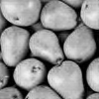 |
This work is licensed under a Creative Commons Attribution 4.0 International License