Function Repository Resource:

LagrangePointData (1.0.0) current version: 1.0.2 »

Source Notebook

Compute properties for the Lagrange points of two orbiting astronomical bodies

Contributed by: Jeff Bryant

ResourceFunction["LagrangePointData"][{entity₁, entity₂},property]

compute the current value of property for entity₁ and entity₂.

ResourceFunction["LagrangePointData"][{entity₁, entity₂},date,property]

compute the value of property on the specified date.

Details and Options

Computations are done in a coordinate system that rotates with the two bodies as they orbit.

The gravitational potential includes terms for the masses of the two bodies in addition to a centripetal term due to the orbital motion.

The "NondimensionalizedPotential" sub‐value of the "GravitationalEffectivePotentialData" property uses MKS units.

The property can be any of the following:

"ContourPlot"

contour plot of the gravitational potential

"ContourPlot3D"

3D contour plot of the gravitational potential

"Distances"

dataset of distances between the bodies and the Lagrange points

"GravitationalEffectivePotentialData"

association of data related to the gravitational potential

"Plot3D"

3D surface plot of the gravitational potential

The distance between the two bodies changes with time, scaling the numbers accordingly.

Options supported by LagrangePointData include:

"EmphasizeSecondaryMassRegion"

False

whether or not to zoom into the area near the secondary mass

TargetUnits

Automatic

units to use only when requesting distances

Additional options vary depending on the property requested ("ContourPlot" supports all the options of ContourPlot, etc.).

The potential can be used to formulate the position and speed of a third body in the system using the following equations of motion: x''-2ωy'==-∂V/∂x, y''+2ωx'==-∂V/∂y.

Examples

Basic Examples (6)

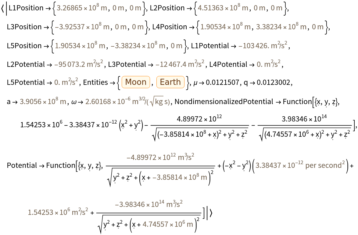
Compute data about the gravitational potential:

In[1]:=

Out[1]=

Find the gravitational potential at a specific 3D point:

In[2]:=

$ResourceFunction["LagrangePointData", ResourceVersion->"1.0.0"][{Entity["Planet", "Earth"], Entity["PlanetaryMoon", "Moon"]}, "GravitationalEffectivePotentialData"]["Potential"][ Quantity[3.44*^8, "Meters"], Quantity[0, "Meters"], Quantity[0, "Meters"]]$

Out[2]=

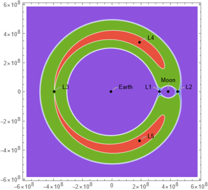
Create a contour plot of the gravitational potential:

In[3]:=

Out[3]=

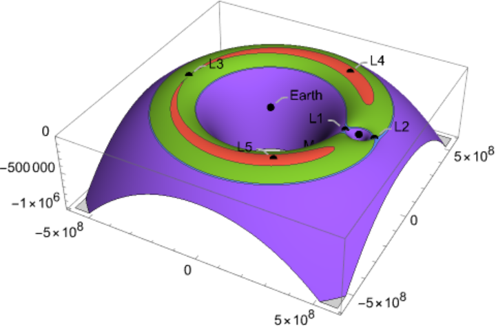
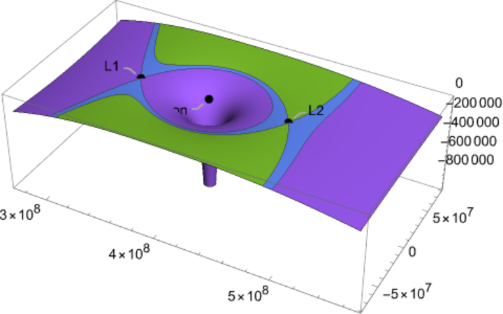
Create a 3D surface plot of the gravitational potential:

In[4]:=

Out[4]=

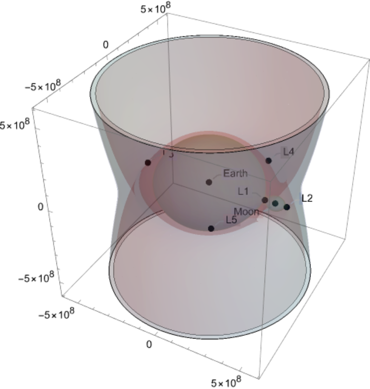
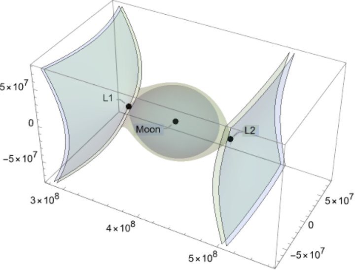
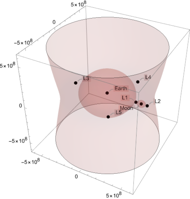
Create a 3D contour plot of the gravitational potential:

In[5]:=

Out[5]=

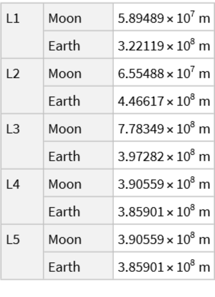
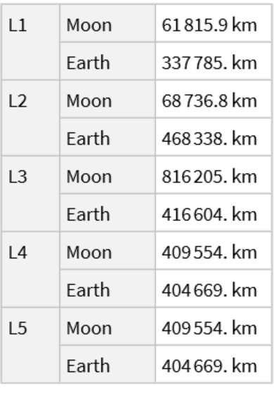
Compute the current distance between both bodies and the various Lagrange points:

In[6]:=

Out[6]=

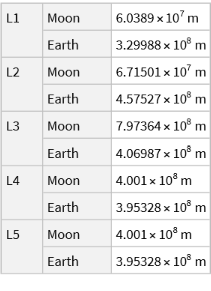
Compute the distance between both bodies and the various Lagrange points on a specified date:

In[7]:=

Out[7]=

Scope (1)

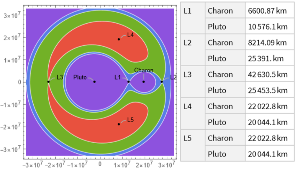
Create a contour plot with distances:

In[8]:=

Out[8]=

Options (3)

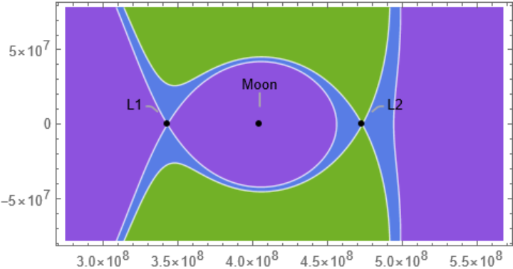
Emphasize the area around the secondary mass:

In[9]:=

Out[9]=

Emphasize the area around the secondary mass:

In[10]:=

Out[10]=

Emphasize the area around the secondary mass:

In[11]:=

Out[11]=

In[12]:=

Out[12]=

Plot the Lagrange points:

In[13]:=

With[{entities = {Entity["Planet", "Earth"], Entity["PlanetaryMoon", "Moon"]}}, ResourceFunction["LagrangePointData"][entities, "ContourPlot3D", Contours -> {QuantityMagnitude[
ResourceFunction["LagrangePointData"][entities, "GravitationalEffectivePotentialData"]["L1Potential"]]}]]

Out[13]=

Applications (4)

Compute the distances of the bodies to the L1 point of the Earth-Moon system:

In[14]:=

Out[14]=

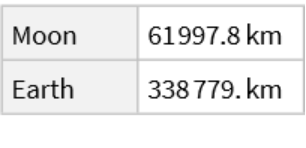
Compute the distance of the Earth to the L1 point of the Earth-Moon system:

In[15]:=

ResourceFunction["LagrangePointData", ResourceVersion->"1.0.0"][{Entity["Planet", "Earth"], Entity["PlanetaryMoon", "Moon"]}, "Distances", TargetUnits -> "Kilometers"]["L1"][Entity["Planet", "Earth"]]

Out[15]=

Compute the distance between the Moon and the L1 point of the Earth-Moon system:

In[16]:=

Out[16]=

Compute the distance between Earth and the Moon:

In[17]:=

Out[17]=

Possible Issues (1)

If the two bodies don't orbit each other, then computations are not applicable:

In[18]:=

Out[18]=

Neat Examples (3)

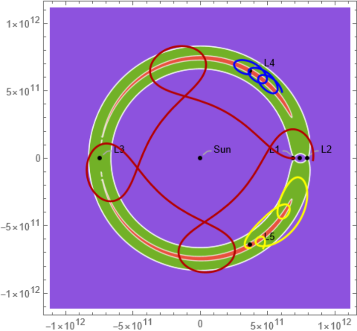
Explore the Lagrange points of the Sun‐Jupiter system:

In[19]:=

${\[Omega], V, L1, L4, L5, cp} = Flatten[{{QuantityMagnitude[#[[1]]], #[[2]][x[t], y[t], z[t]], QuantityMagnitude[#[[3]]], QuantityMagnitude[#[[4]]], QuantityMagnitude[#[[5]]]} &@ Lookup[#[[1]], {"\[Omega]", "NondimensionalizedPotential", "L1Position", "L4Position", "L5Position"}], #[[2]]} &@ ResourceFunction["LagrangePointData", ResourceVersion->"1.0.0"][{Entity["Star", "Sun"], Entity["Planet", "Jupiter"]}, {"GravitationalEffectivePotentialData", "ContourPlot"}], 1] /. z[t] -> 0;$

Solve the equations of motion for a particle starting at the L1 point and moving in the -x‐direction and -y‐direction over a period of about 31 years (1,000,000,000 seconds):

In[20]:=

$L1sols = NDSolve[{x''[t] - 2 \[Omega] y'[t] == -D[V, x[t]], y''[t] + 2 \[Omega] x'[t] == -D[V, y[t]], x'[0] == -5000., y'[0] == -300., x[0] == L1[[1]], y[0] == L1[[2]], z[0] == L1[[3]]}, {x, y}, {t, 0, 1000000000}];$

Solve the equations of motion for particle starting near the L4 and L5 points with different initial velocities:

In[21]:=

$L4sols = NDSolve[{x''[t] - 2 \[Omega] y'[t] == -D[V, x[t]], y''[t] + 2 \[Omega] x'[t] == -D[V, y[t]], x'[0] == -1000., y'[0] == -300., x[0] == L4[[1]], y[0] == L4[[2]] - 20000000000, z[0] == L4[[3]]}, {x, y}, {t, 0, 1000000000}];$

In[22]:=

$L5sols = NDSolve[{x''[t] - 2 \[Omega] y'[t] == -D[V, x[t]], y''[t] + 2 \[Omega] x'[t] == -D[V, y[t]], x'[0] == -1000., y'[0] == -300., x[0] == L5[[1]], y[0] == L5[[2]] - 20000000000, z[0] == L5[[3]]}, {x, y}, {t, 0, 1000000000}];$

In[23]:=

In[24]:=

In[25]:=

In[26]:=

Out[26]=

Version History

1.0.2 – 27 October 2023
1.0.1 – 27 September 2023
1.0.0 – 22 September 2023

Source Metadata

Citation:
S Ciulli and C Sebu 2008 J. Phys. A: Math. Theor. 41 335201

License Information

This work is licensed under a Creative Commons Attribution 4.0 International License

Wolfram Function Repository

LagrangePointData (1.0.0) current version: 1.0.2 »

Details and Options