Details and Options
Computations are done in a coordinate system that rotates with the two primary bodies as they orbit.
In the coordinate system used, the origin is at the center of mass of the system and the orbiting bodies orbit in the x‐y plane with the z‐axis perpendicular to that plane.
The positive x‐direction is in the direction of the smaller mass.
The positive y‐direction follows a right‐hand rule convention.
The gravitational effective potential includes terms for the masses of the two bodies in addition to a centripetal term due to the orbital motion.
The distance between the two bodies changes with time, scaling the numbers accordingly.
For a given date, the gravitational effective potential assumes a circular orbit of entity1 and entity2 using the distance on that date (a) as the distance between the bodies.
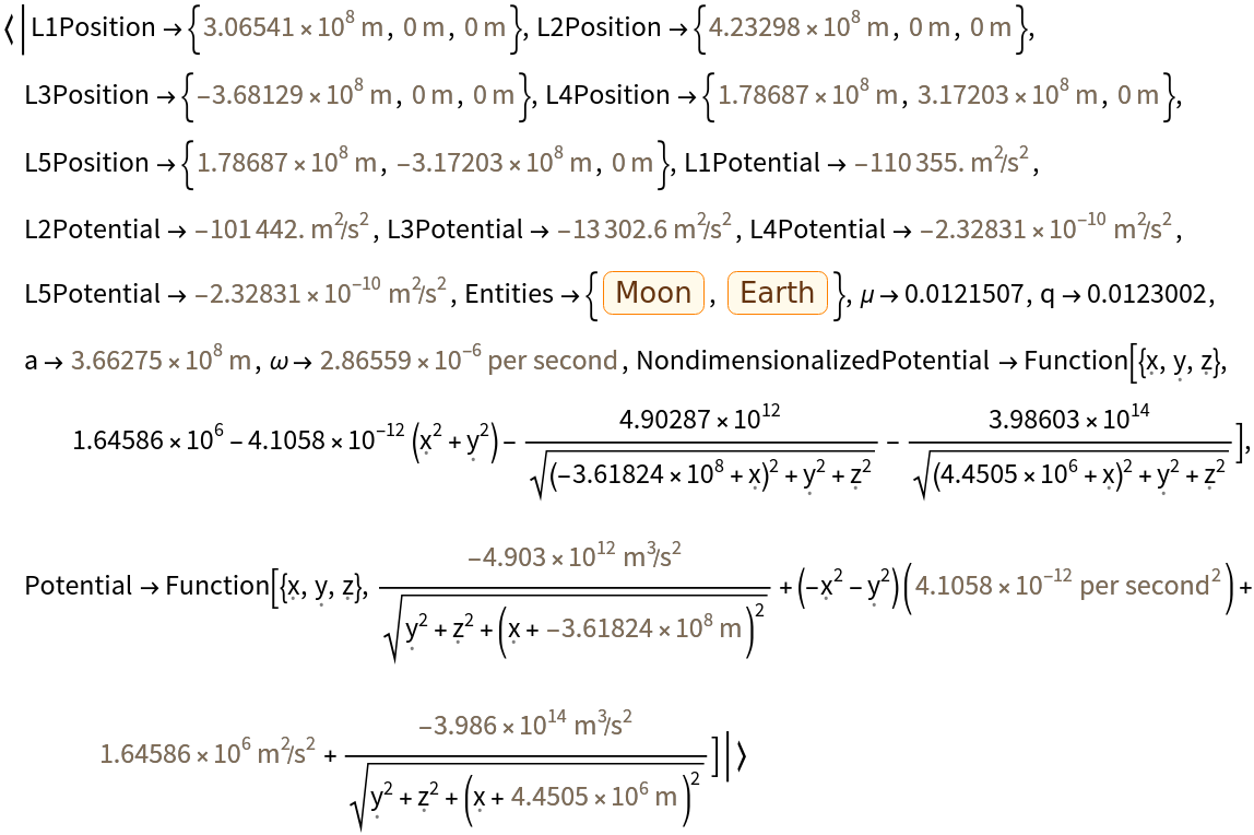
The following keys can be seen in the results:
| q | the mass ratio, Msecondary/Mprimary |
| μ | the reduced mass,Msecondary/(Mprimary + Msecondary) |
| a | the distance between entity1 and entity2 |
| ω | the angular velocity of the orbit |
The "NondimensionalizedPotential" sub‐value of the "GravitationalEffectivePotentialData" property uses SI base units.
The property can be any of the following:
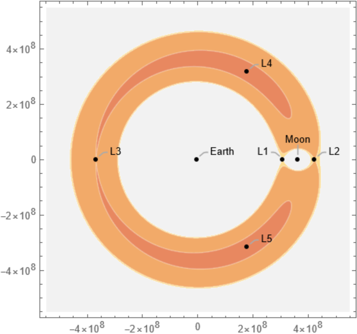
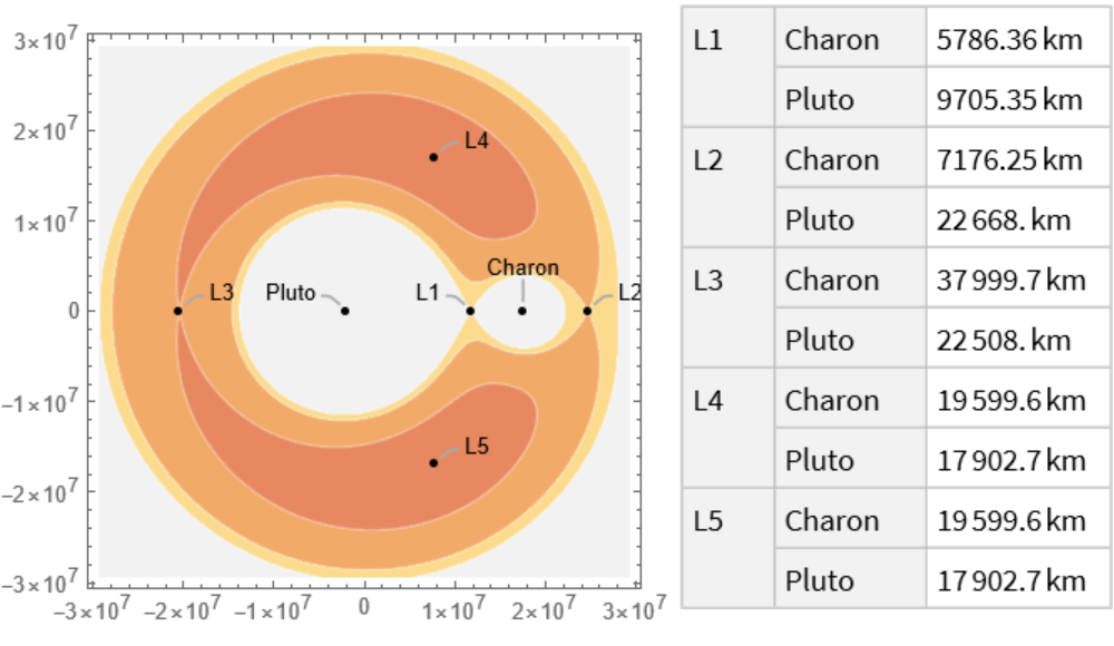
| "ContourPlot" | contour plot of the gravitational effective potential |
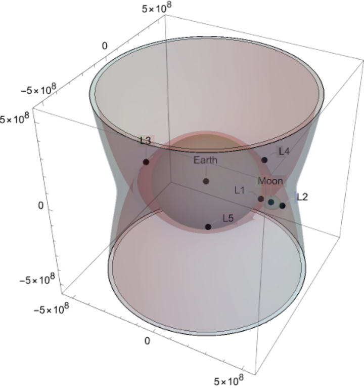
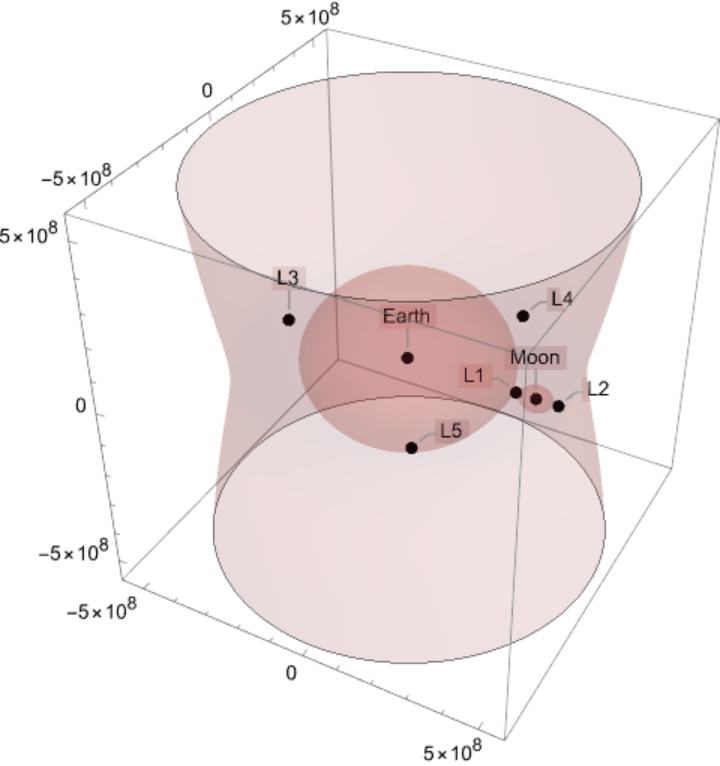
| "ContourPlot3D" | 3D contour plot of the gravitational effective potential |
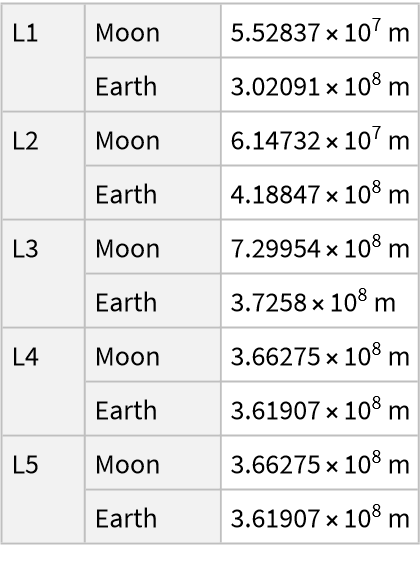
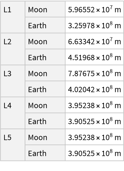
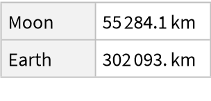
| "Distances" | dataset of distances between the bodies and the Lagrange points |
| "GravitationalEffectivePotentialData" | association of data related to the gravitational effective potential |
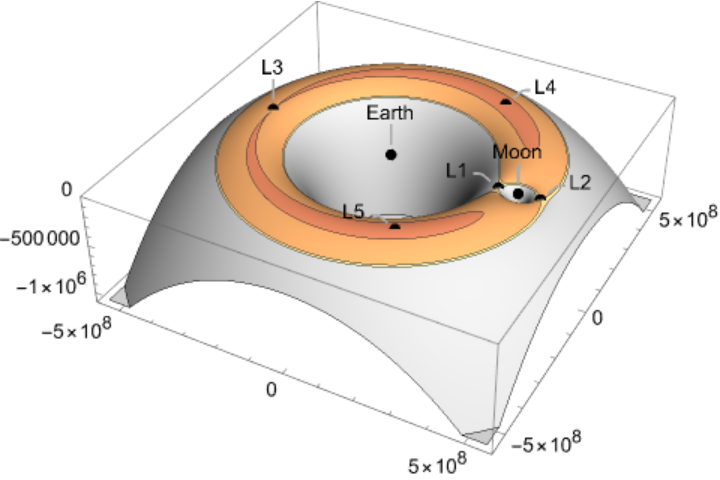
| "Plot3D" | 3D surface plot of the gravitational effective potential |
Options supported by LagrangePointData include:
| "EmphasizeSecondaryMassRegion" | False | whether or not to zoom into the area near the secondary mass |
| TargetUnits | Automatic | units to use only when requesting distances |
Additional options vary depending on the property requested ("ContourPlot" supports all the options of
ContourPlot, etc.).
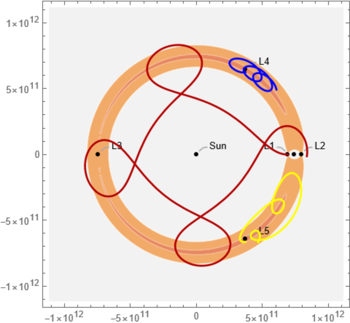
The potential (V) can be used to formulate the position and speed of a third body in the system using the following equations of motion: x''-2ωy'==-∂V/∂x, y''+2ωx'==-∂V/∂y.
![ResourceFunction[
"LagrangePointData", ResourceSystemBase -> "https://www.wolframcloud.com/obj/resourcesystem/api/1.0"][{Entity["Planet", "Earth"], Entity["PlanetaryMoon", "Moon"]}, "GravitationalEffectivePotentialData"]](https://www.wolframcloud.com/obj/resourcesystem/images/5b5/5b5e56d3-2ec1-4f5b-a09d-9dd802a61a86/64bd54cb8a97a5f5.png)
![ResourceFunction[
"LagrangePointData", ResourceSystemBase -> "https://www.wolframcloud.com/obj/resourcesystem/api/1.0"][{Entity["Planet", "Earth"], Entity["PlanetaryMoon", "Moon"]}, "GravitationalEffectivePotentialData"]["Potential"][
Quantity[3.44*^8, "Meters"], Quantity[0, "Meters"], Quantity[0, "Meters"]]](https://www.wolframcloud.com/obj/resourcesystem/images/5b5/5b5e56d3-2ec1-4f5b-a09d-9dd802a61a86/26cd1c42311357f6.png)
![ResourceFunction[
"LagrangePointData", ResourceSystemBase -> "https://www.wolframcloud.com/obj/resourcesystem/api/1.0"][{Entity["Planet", "Earth"], Entity["PlanetaryMoon", "Moon"]}, DateObject[{2024, 7, 16, 0, 0, 0}, TimeZone -> "America/Chicago"], "Distances"]](https://www.wolframcloud.com/obj/resourcesystem/images/5b5/5b5e56d3-2ec1-4f5b-a09d-9dd802a61a86/4803d3246ddbb0c0.png)
![Grid[{ResourceFunction[
"LagrangePointData", ResourceSystemBase -> "https://www.wolframcloud.com/obj/resourcesystem/api/1.0"][{Entity["MinorPlanet", "Pluto"], Entity["PlanetaryMoon", "Charon"]}, {"ContourPlot", "Distances"}, ImageSize -> 300, TargetUnits -> "Kilometers"]}]](https://www.wolframcloud.com/obj/resourcesystem/images/5b5/5b5e56d3-2ec1-4f5b-a09d-9dd802a61a86/3aa5aa5eaef654a4.png)
![ResourceFunction[
"LagrangePointData", ResourceSystemBase -> "https://www.wolframcloud.com/obj/resourcesystem/api/1.0"][{Entity["Planet", "Earth"], Entity["PlanetaryMoon", "Moon"]}, "ContourPlot", "EmphasizeSecondaryMassRegion" -> True]](https://www.wolframcloud.com/obj/resourcesystem/images/5b5/5b5e56d3-2ec1-4f5b-a09d-9dd802a61a86/2cf4fead61e94e50.png)
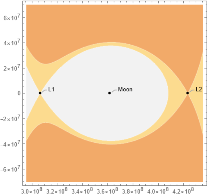
![ResourceFunction[
"LagrangePointData", ResourceSystemBase -> "https://www.wolframcloud.com/obj/resourcesystem/api/1.0"][{Entity["Planet", "Earth"], Entity["PlanetaryMoon", "Moon"]}, "Plot3D", "EmphasizeSecondaryMassRegion" -> True]](https://www.wolframcloud.com/obj/resourcesystem/images/5b5/5b5e56d3-2ec1-4f5b-a09d-9dd802a61a86/0031547860a87692.png)
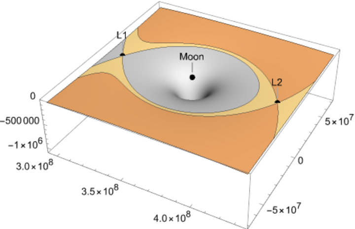
![ResourceFunction[
"LagrangePointData", ResourceSystemBase -> "https://www.wolframcloud.com/obj/resourcesystem/api/1.0"][{Entity["Planet", "Earth"], Entity["PlanetaryMoon", "Moon"]}, "ContourPlot3D", "EmphasizeSecondaryMassRegion" -> True]](https://www.wolframcloud.com/obj/resourcesystem/images/5b5/5b5e56d3-2ec1-4f5b-a09d-9dd802a61a86/0630af620c80e75a.png)
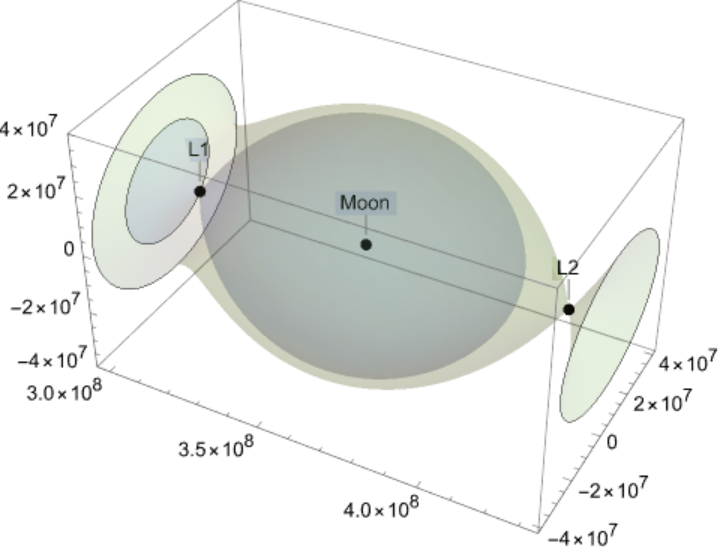
![ResourceFunction[
"LagrangePointData", ResourceSystemBase -> "https://www.wolframcloud.com/obj/resourcesystem/api/1.0"][{Entity["Planet", "Earth"], Entity["PlanetaryMoon", "Moon"]}, "Distances", TargetUnits -> "Kilometers"]](https://www.wolframcloud.com/obj/resourcesystem/images/5b5/5b5e56d3-2ec1-4f5b-a09d-9dd802a61a86/34e7c91770362f29.png)
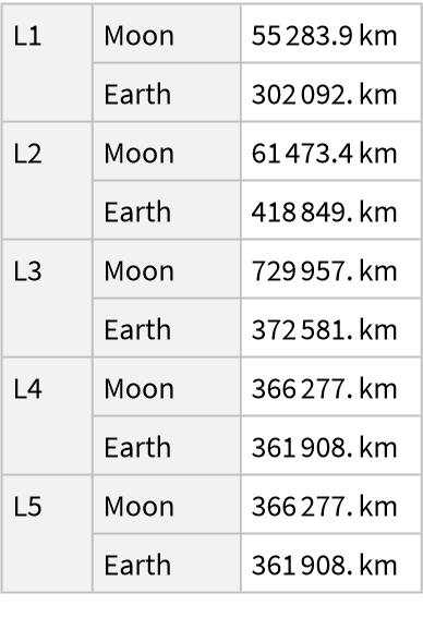
![With[{entities = {Entity["Planet", "Earth"], Entity["PlanetaryMoon", "Moon"]}}, ResourceFunction[
"LagrangePointData", ResourceSystemBase -> "https://www.wolframcloud.com/obj/resourcesystem/api/1.0"][entities, "ContourPlot3D", Contours -> {QuantityMagnitude[
ResourceFunction[
"LagrangePointData", ResourceSystemBase -> "https://www.wolframcloud.com/obj/resourcesystem/api/1.0"][entities, "GravitationalEffectivePotentialData"]["L1Potential"]]}]]](https://www.wolframcloud.com/obj/resourcesystem/images/5b5/5b5e56d3-2ec1-4f5b-a09d-9dd802a61a86/66c9521bd3e9263c.png)
![ResourceFunction[
"LagrangePointData", ResourceSystemBase -> "https://www.wolframcloud.com/obj/resourcesystem/api/1.0"][{Entity["Planet", "Earth"], Entity["PlanetaryMoon", "Moon"]}, "Distances", TargetUnits -> "Kilometers"]["L1"]](https://www.wolframcloud.com/obj/resourcesystem/images/5b5/5b5e56d3-2ec1-4f5b-a09d-9dd802a61a86/7694dbbc1d8272d9.png)
![ResourceFunction[
"LagrangePointData", ResourceSystemBase -> "https://www.wolframcloud.com/obj/resourcesystem/api/1.0"][{Entity["Planet", "Earth"], Entity["PlanetaryMoon", "Moon"]}, "Distances", TargetUnits -> "Kilometers"]["L1"][Entity["Planet", "Earth"]]](https://www.wolframcloud.com/obj/resourcesystem/images/5b5/5b5e56d3-2ec1-4f5b-a09d-9dd802a61a86/3156d4e1f9d83f9f.png)
![ResourceFunction[
"LagrangePointData", ResourceSystemBase -> "https://www.wolframcloud.com/obj/resourcesystem/api/1.0"][{Entity["Planet", "Earth"], Entity["PlanetaryMoon", "Moon"]}, "Distances", TargetUnits -> "Kilometers"]["L1"][Entity["PlanetaryMoon", "Moon"]]](https://www.wolframcloud.com/obj/resourcesystem/images/5b5/5b5e56d3-2ec1-4f5b-a09d-9dd802a61a86/2ada38ae984eabc7.png)
![ResourceFunction[
"LagrangePointData", ResourceSystemBase -> "https://www.wolframcloud.com/obj/resourcesystem/api/1.0"][{Entity["Planet", "Earth"], Entity["Planet", "Mars"]}, "GravitationalEffectivePotentialData"]](https://www.wolframcloud.com/obj/resourcesystem/images/5b5/5b5e56d3-2ec1-4f5b-a09d-9dd802a61a86/676a7b00089f4110.png)
![{\[Omega], V, L1, L4, L5, cp} = Flatten[{{QuantityMagnitude[#[[1]]], #[[2]][x[t], y[t], z[t]], QuantityMagnitude[#[[3]]], QuantityMagnitude[#[[4]]], QuantityMagnitude[#[[5]]]} &@
Lookup[#[[1]], {"\[Omega]", "NondimensionalizedPotential", "L1Position", "L4Position", "L5Position"}], #[[2]]} &@
ResourceFunction[
"LagrangePointData", ResourceSystemBase -> "https://www.wolframcloud.com/obj/resourcesystem/api/1.0"][{Entity["Star", "Sun"], Entity["Planet", "Jupiter"]}, {"GravitationalEffectivePotentialData", "ContourPlot"}], 1] /. z[t] -> 0;](https://www.wolframcloud.com/obj/resourcesystem/images/5b5/5b5e56d3-2ec1-4f5b-a09d-9dd802a61a86/528c9e59c0a3d396.png)
![L1sols = NDSolve[{x''[t] - 2 \[Omega] y'[t] == -D[V, x[t]], y''[t] + 2 \[Omega] x'[t] == -D[V, y[t]], x'[0] == -5000., y'[0] == -300., x[0] == L1[[1]], y[0] == L1[[2]], z[0] == L1[[3]]}, {x, y}, {t, 0, 1000000000}];](https://www.wolframcloud.com/obj/resourcesystem/images/5b5/5b5e56d3-2ec1-4f5b-a09d-9dd802a61a86/33ee8c316a130d58.png)
![L4sols = NDSolve[{x''[t] - 2 \[Omega] y'[t] == -D[V, x[t]], y''[t] + 2 \[Omega] x'[t] == -D[V, y[t]], x'[0] == -1000., y'[0] == -300., x[0] == L4[[1]], y[0] == L4[[2]] - 20000000000, z[0] == L4[[3]]}, {x, y}, {t, 0, 1000000000}];](https://www.wolframcloud.com/obj/resourcesystem/images/5b5/5b5e56d3-2ec1-4f5b-a09d-9dd802a61a86/2bae4a486f863216.png)
![L5sols = NDSolve[{x''[t] - 2 \[Omega] y'[t] == -D[V, x[t]], y''[t] + 2 \[Omega] x'[t] == -D[V, y[t]], x'[0] == -1000., y'[0] == -300., x[0] == L5[[1]], y[0] == L5[[2]] - 20000000000, z[0] == L5[[3]]}, {x, y}, {t, 0, 1000000000}];](https://www.wolframcloud.com/obj/resourcesystem/images/5b5/5b5e56d3-2ec1-4f5b-a09d-9dd802a61a86/380624fad0bbad28.png)
![L1path = ParametricPlot[Evaluate[{x[t], y[t]} /. L1sols], {t, 0, 1000000000},
PlotStyle -> Darker[Red, .3]];](https://www.wolframcloud.com/obj/resourcesystem/images/5b5/5b5e56d3-2ec1-4f5b-a09d-9dd802a61a86/28343cb71cdf894c.png)
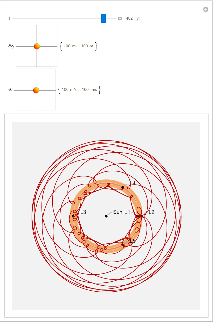
![Manipulate[
Module[{sol, L4 = Most[L4]}, sol = NDSolve[{x''[t] - 2 \[Omega] y'[t] == -D[V, x[t]], y''[t] + 2 \[Omega] x'[t] == -D[V, y[t]], x'[0] == v0[[1]], y'[0] == v0[[2]], x[0] == L4[[1]] + \[Delta]xy[[1]], y[0] == L4[[2]] + \[Delta]xy[[2]]}, {x, y}, {t, 0, 10^T}];
Show[{cp, ParametricPlot[Evaluate[({x[t], y[t]}) /. sol], {t, 0, 10^T}, PlotStyle -> Directive[Darker[Red, .3], Thickness[0.003]], Frame -> True, Axes -> False]}, PlotRangePadding -> 1*^12, Frame -> False, Axes -> False, Background -> GrayLevel[.95]]], Row[{Control[{{T, 10.2, "T"}, 3, 11}], " ", Dynamic[Quantity[Round[10^T/3.28725`*^7, 0.1], "Years"]]}], Row[{Control[{{\[Delta]xy, {100, 100}}, 10^6 {-1, -1}, 10^6 {1, 1}}],
" ", Dynamic[Quantity[Round[\[Delta]xy, 0.1], "Meters"]]}], Row[{Control[{{v0, {575, -300}}, 10^4 {-1, -1}, 10^4 {1, 1}}], " ", Dynamic[Quantity[Round[\[Delta]xy, 0.1], "Meters"/"Seconds"]]}], SynchronousUpdating -> False]](https://www.wolframcloud.com/obj/resourcesystem/images/5b5/5b5e56d3-2ec1-4f5b-a09d-9dd802a61a86/02f882164368d5cd.png)
