Basic Examples (2) 

The points forming a 1^st-step Koch curve:

In[1]:=

Out[1]=

A 1^st-step Koch curve visualization:

In[2]:=

Out[2]=

Visualizations of the 2^nd through 5^th-step Koch curves:

In[3]:=

Out[3]=

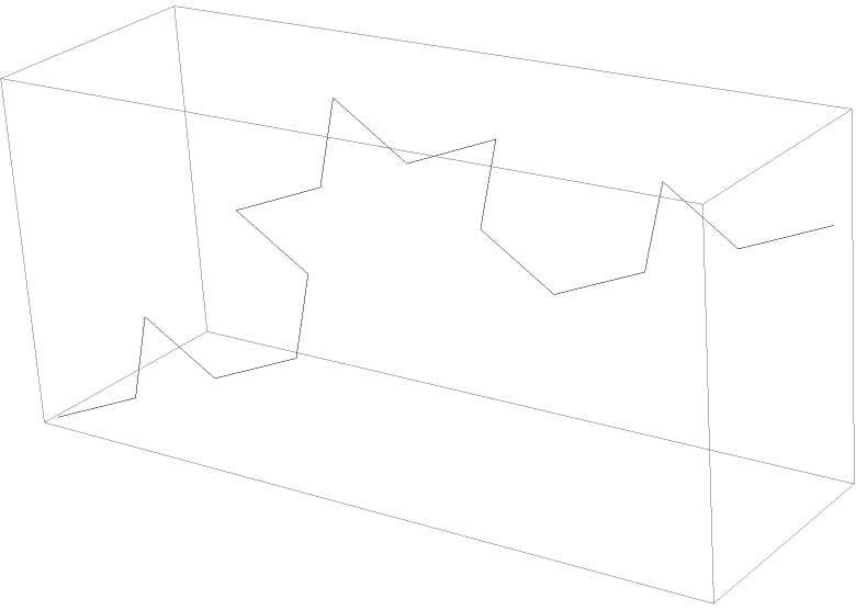
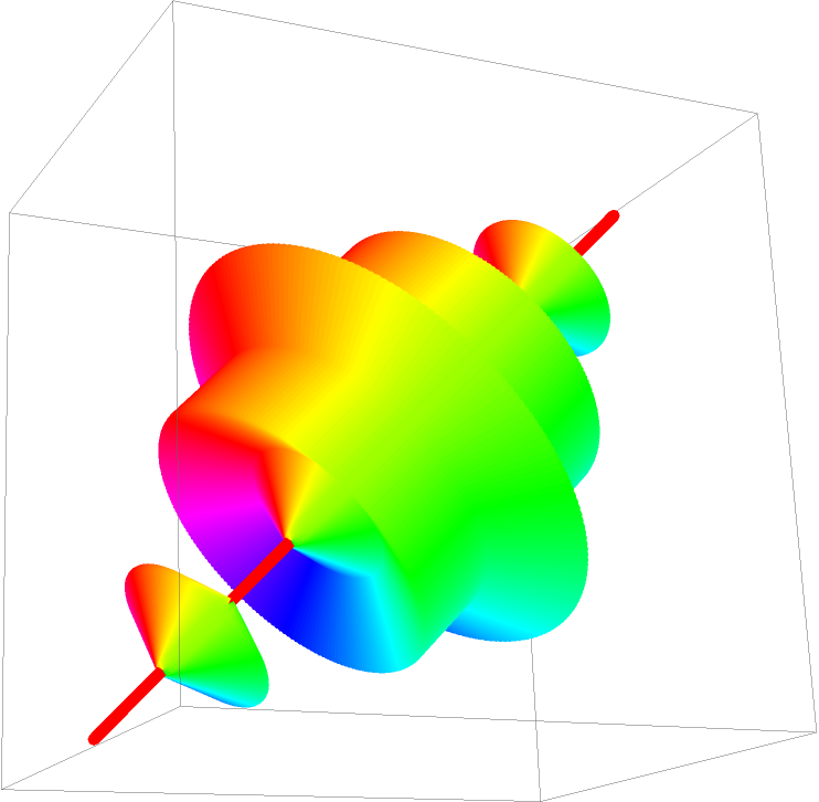
A 2^nd-step Koch curve in 3 dimensions:

In[4]:=

Out[4]=

Scope (5) 

Form Koch curves over a 2D list of points:

In[5]:=

Out[5]=

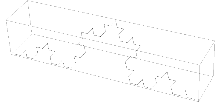
Form Koch curves over a 3D list of points:

In[6]:=

Out[6]=

Change the path direction of the 2D Koch curve:

In[7]:=

Out[7]=

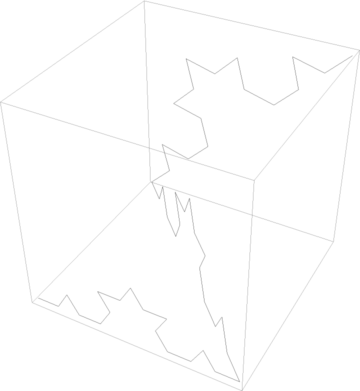
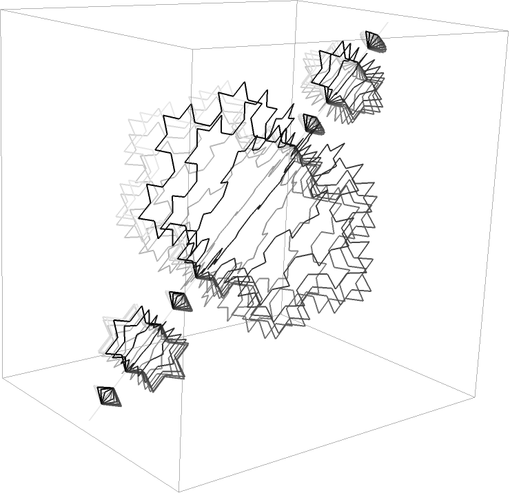
Change the path angle of the 3D Koch curve:

In[8]:=

Out[8]=

A representation of how the angle rotates the 3D Koch curve, where the 0 angle is in black:

In[9]:=

Out[9]=

The 0^th-step Koch Curve does not introduce any new points:

In[10]:=

Out[10]=

Options (2) 

Setting "ExactValues" to False causes the output to be imprecise:

In[11]:=

Out[11]=

Imprecise outputs are much faster to compute:

In[12]:=

Out[12]=

In[13]:=

Out[13]=

Applications (2) 

Form a Koch snowflake by specifying the corner points:

In[14]:=

Out[14]=

Invert the Koch snowflake:

In[15]:=

Out[15]=

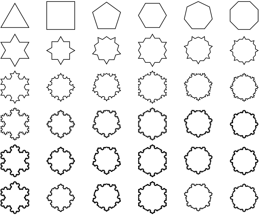
A matrix of the first six steps of Koch snowflakes from the first six regular polygons:

In[16]:=

Out[16]=

Properties and Relations (1) 

The Koch snowflake can be generated with either KochCurve or KochCurvePoints:

In[17]:=

Out[17]=

In[18]:=

Out[18]=

Possible Issues (1) 

If a point or the value of the orientation is inexact, then parts of the output will return inexact:

In[19]:=

Out[19]=

In[20]:=

Out[20]=

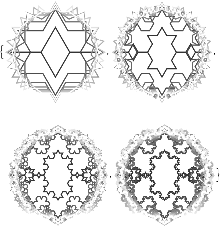
Neat Examples (4) 

Increasing the density of lines gives the impression of a solid object:

In[21]:=

Out[21]=

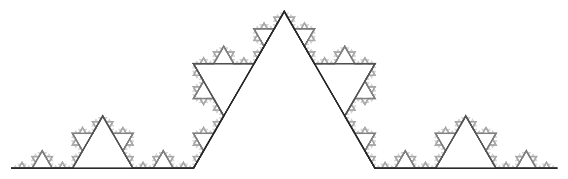
Visualize the increasing detail of higher-step Koch curves:

In[22]:=

Out[22]=

Apply the Koch Curve to other named curves:

In[23]:=

Out[23]=

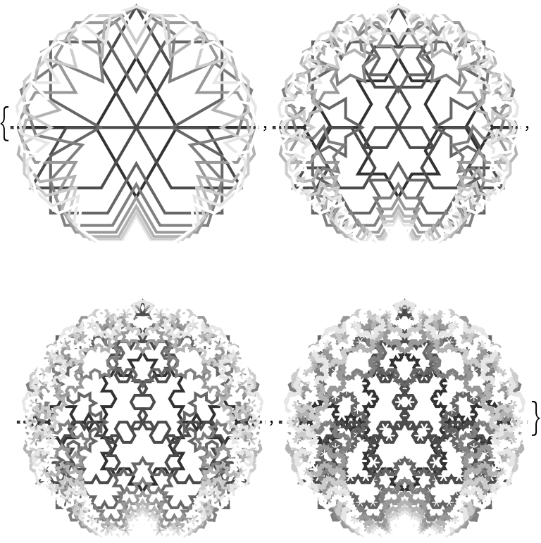
An overlap of the Koch Snowflakes generated from the first 10 regular polygons:

In[24]:=

Out[24]=

The same Koch Snowflakes when the orientation is reversed:

In[25]:=

Out[25]=