Basic Examples (5)
Define a geometric Brownian motion stochastic process:
Get the arithmetic Brownian motion via a logarithmic transformation:
Mean and variance of the transformed process:
Start with a Wiener process:
In a square transformation of this process, a particular branch is picked in the inverse mapping:
Define a 2D process with the noise as a matrix:
Two variable linear transformation of the process:
Start with a Wiener process:
Perform an exponential transformation:
Create a geometric Brownian motion process:
Reciprocal transformation of the process:
Scope (4)
Create a particular Ito process:
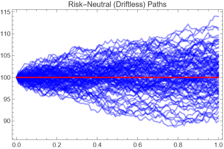
Explicit time-dependent transformation:
Start with a driftless process:
Calculate the drift of the transformation under the variable change z = tanh(x):
Start with a 2D Wiener process:
Transform the process to polar coordinates such that the initial zero drift becomes non zero and radial dependent in polar coordinates:
Start with a 3D Wiener process:
Transform the process from Cartesian to ParabolicCylindrical coordinates using a long name convention:
Options (4)
Define a 1D Wiener process:
Perform a trigonometric change of variables, because of the periodic nature of the transformation is not possible to get a unique solution:
Using the assumption 0<x<π, we select one branch:
Using the assumption -π<x<0, we get a different branch that has a sign flip in the diffusion:
Applications (17)
Mean shifting Ornstein-Uhlenbeck (4)
Define the OrnsteinUhlenbeck process:
Compute mean and variance of the process:
Perform the variable change y=x-μ:
Check the mean and variance, the mean got shifted but the process remains OrnsteinUhlenbeck:
Risk-neutral measure (GBM model) (3)
Define a geometric Brownian motion process modeling a stock price:
Find the discounted stock price via the transformation S = ⅇ-r tx, S is a martingale:
Show a path simulation, setting σ = 0.05 and x0 = 100:
Noisy oscillator (4)
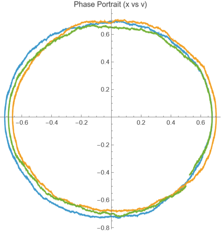
Define a process representing a noisy oscillator, with drift in velocity related to position (as in Hooke's law), with added diffusion only in velocity:
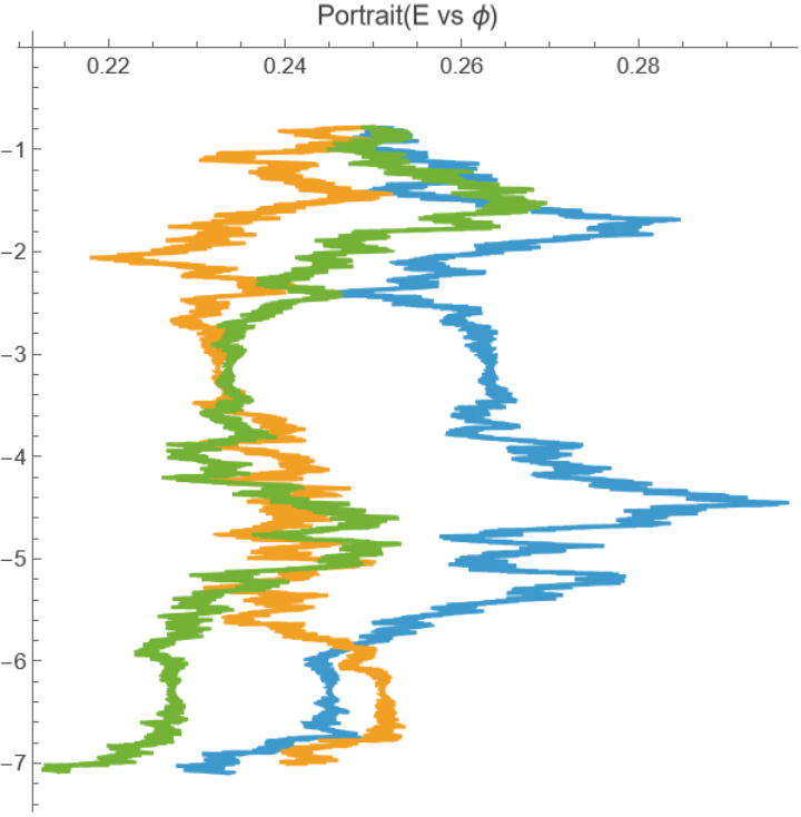
Transforming to E and ϕ variables (energy and phase):
Show a path simulation with σ=0.03,x0=0.5,v0=-0.5. Plotting the phase portrait we get deformed circular paths:
In energy-phase space the same parameters create noisy paths:
Quantum State Diffusion (6)
Define a stochastic differential equation in Cartesian coordinates, this process was obtained from Quantum State Diffusion for some density matrix ρ and Lindblad jump operator L=σz:
Perform change of variables to spherical coordinates which are more appropriate to the geometry of the state space:
Assign parameters. The initial state is on the surface of the Bloch sphere (r =1, θ=π/3, ϕ = π/3):
Generate 100 realizations of the transformed process using simulation time γ/ωx:
Calculate Bloch vector trajectories:
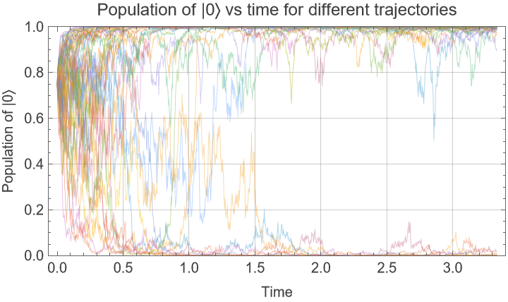
Population of |0〉 can be calculated as  , show some trajectories and how they converge towards the poles:
Possible Issues (2)
If no initial state is supplied when creating a process the default is 0 for each state variable:
Some initial conditions may be undefined under the variable transformation, in this case the origin:
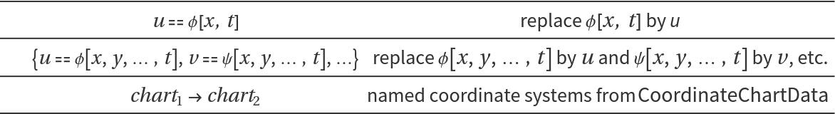


![paths = RandomFunction[
transformedProc /. {\[Sigma] -> 0.05, x0 -> 100}, {0, 1, 0.01}, 100];
cleanedPaths = paths["Paths"] /. {t_, {v_}} :> {t, v};
ListLinePlot[cleanedPaths, PlotStyle -> Directive[Opacity[0.4`], Blue],
PlotLabel -> "Risk-Neutral (Driftless) Paths", AxesLabel -> {"Time (T)", "Value (Y)"}, Frame -> True, Epilog -> {Red, Thick, Line[{{0, 100}, {1, 100}}]} ]](https://www.wolframcloud.com/obj/resourcesystem/images/2c7/2c7d8c8d-85ab-437d-a1e0-417e2c898ac2/28a3c9d19731b760.png)

![paths = RandomFunction[(oscillator /. {\[Sigma] -> 0.03, x0 -> 0.5, v0 -> -0.5}), {0, 2 \[Pi], 0.001}, 3];
data = paths["Paths"][[All, All, 2]];
ListLinePlot[data, AspectRatio -> 1, PlotRange -> All, PlotLabel -> "Phase Portrait (x vs v)"]](https://www.wolframcloud.com/obj/resourcesystem/images/2c7/2c7d8c8d-85ab-437d-a1e0-417e2c898ac2/7fc004150c3fd4c2.png)
![paths = RandomFunction[(transformed /. {\[Sigma] -> 0.03, x0 -> 0.5, v0 -> -0.5}), {0, 2 \[Pi], 0.001}, 3];
data = paths["Paths"][[All, All, 2]];
ListLinePlot[data, AspectRatio -> 1, PlotRange -> All, PlotLabel -> "Portrait(E vs \[Phi])"]](https://www.wolframcloud.com/obj/resourcesystem/images/2c7/2c7d8c8d-85ab-437d-a1e0-417e2c898ac2/6d73e2c626cf3aca.png)
![procCartesian = ItoProcess[{{-2 x \[Gamma], -2 y \[Gamma] - z \[Omega]x, y \[Omega]x}, {-2 x z Sqrt[\[Gamma]], -2 y z Sqrt[\[Gamma]], 2 (1 - z^2) Sqrt[\[Gamma]]}}, {{x, y, z}, {x0, y0, z0}}, t];](https://www.wolframcloud.com/obj/resourcesystem/images/2c7/2c7d8c8d-85ab-437d-a1e0-417e2c898ac2/0ea47c983f11afee.png)

![procSpherical = procSpherical /. Join[Thread[{x0, y0, z0} -> FromSphericalCoordinates[{1, \[Pi]/3, \[Pi]/3}]], {\[Gamma] -> 1, \[Omega]x -> 0.3}];](https://www.wolframcloud.com/obj/resourcesystem/images/2c7/2c7d8c8d-85ab-437d-a1e0-417e2c898ac2/09d699b14d934a6d.png)
![blochVectorTrajectoriesCollapse = MapAt[Apply[#1 {Cos[#3] Sin[#2], Sin[#3] Sin[#2], Cos[#2]} &], trajectoriesSpherical["ValueList"], {All, All}];](https://www.wolframcloud.com/obj/resourcesystem/images/2c7/2c7d8c8d-85ab-437d-a1e0-417e2c898ac2/6a8b5951e61ed086.png)