Wolfram Function Repository
Instant-use add-on functions for the Wolfram Language
Function Repository Resource:
Decompose a matrix into Independent Component Analysis matrix factors
ResourceFunction["IndependentComponentAnalysis"][mat,k] decomposes the matrix mat into k components. | |
ResourceFunction["IndependentComponentAnalysis"][mat,k,opts] decomposes mat using the options opts. |
| "InitialUnmixingMatrix" | Automatic | initial un-mixing matrix |
| "NegEntropyFactor" | 1 | negative entropy factor |
| "NonGaussianityFunction" | Automatic | non-Gaussianity measure function |
| "RowNorm" | False | whether to normalize the matrix rows at each step |
| MaxSteps | 200 | maximum steps of the ICA interation process |
| PrecisionGoal | 6 | precision goal |
Here is a random integer matrix:
| In[1]:= | ![SeedRandom[7]
mat = RandomInteger[10, {4, 3}];
MatrixForm[mat]](https://www.wolframcloud.com/obj/resourcesystem/images/c3f/c3fea6ef-e925-4a13-832e-bc1ebe467c12/5efa85c9146716d9.png) |
| Out[3]= |  |
Here are the Independent Component Analysis matrix factors:
| In[4]:= |
| Out[4]= |  |
Here is the matrix product of the obtained factors:
| In[5]:= |
| Out[8]= |  |
Here is a random matrix with its first two columns having much larger magnitudes than the rest:
| In[9]:= | ![SeedRandom[232];
mat = RandomReal[{10, 100}, {10, 2}];
mat2 = RandomReal[{-10, 10}, {10, 7}];
mat = ArrayPad[mat, {{0, 0}, {0, 5}}] + mat2;](https://www.wolframcloud.com/obj/resourcesystem/images/c3f/c3fea6ef-e925-4a13-832e-bc1ebe467c12/1c22b874445d71a5.png) |
Plot the values:
| In[10]:= |
| Out[10]= | 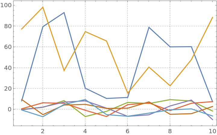 |
Compute the ICA matrix factors:
| In[11]:= |
Here is the relative error of the approximation by the obtained matrix factorization:
| In[12]:= |
| Out[12]= |
Here is the relative error for the first three columns:
| In[13]:= |
| Out[13]= |
Here are comparison plots:
| In[14]:= | ![Block[{opts = {PlotRange -> All, ImageSize -> 250, PlotTheme -> "Detailed"}},
Row[{ListLinePlot[Transpose[mat], opts, PlotLabel -> "Orginal"], ListLinePlot[Transpose[A . S], opts, PlotLabel -> "Reconstructed"]}]
]](https://www.wolframcloud.com/obj/resourcesystem/images/c3f/c3fea6ef-e925-4a13-832e-bc1ebe467c12/771b4715e47b6082.png) |
| Out[14]= | 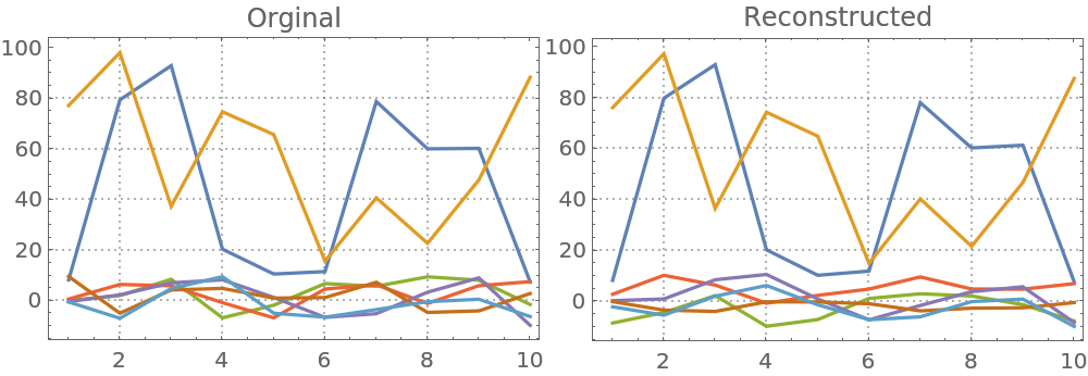 |
Using the option "InitialUnmixingMatrix", we can influence the results by providing initial un-mixing matrix for ICA's iteration process. Here we compute ICA with different initial un-mixing matrices:
| In[15]:= | ![k = 3;
SeedRandom[8];
res = Association[
MapThread[
Row[{#2, ":", Spacer[2], If[MatrixQ[#], MatrixForm[#1], ToString[#1]]}] -> ResourceFunction["IndependentComponentAnalysis"][mat, k, "InitialUnmixingMatrix" -> #1] &, {{Automatic, Automatic, RandomVariate[NormalDistribution[1, 10], {k, k}], SingularValueDecomposition[mat, k][[2]]}, Range[4]}]];](https://www.wolframcloud.com/obj/resourcesystem/images/c3f/c3fea6ef-e925-4a13-832e-bc1ebe467c12/04ccd7172101abf8.png) |
Plot the results:
| In[16]:= | ![Grid[KeyValueMap[{#1, ListLinePlot[Transpose[#2[[1]]], PlotRange -> All, ImageSize -> 250, PlotTheme -> "Detailed"]} &, res], Alignment -> {Center, Left}]](https://www.wolframcloud.com/obj/resourcesystem/images/c3f/c3fea6ef-e925-4a13-832e-bc1ebe467c12/129b9f3efe870241.png) |
| Out[16]= | 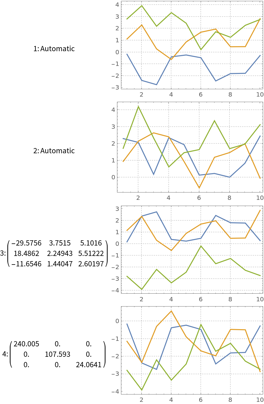 |
ICA is essentially a Gram-Schmidt process that considers two signals to be orthogonal if their difference is Gaussian noise.
Here we compute ICA with different non-Gaussianity measure functions:
| In[17]:= | ![res = Association[
# -> BlockRandom[
SeedRandom[22];
ResourceFunction["IndependentComponentAnalysis"][mat, 3, "NonGaussianityFunction" -> #, MaxSteps -> 2]
] & /@ {Log[
Cosh[#]] &, -Exp[-#^2/2] &, (Log[Cosh[1.2 #]]/1.2 &)}];](https://www.wolframcloud.com/obj/resourcesystem/images/c3f/c3fea6ef-e925-4a13-832e-bc1ebe467c12/655e2bc832a5a9e1.png) |
Plot the results:
| In[18]:= | ![Grid[KeyValueMap[{#1[x], ListLinePlot[Transpose[#2[[1]]], PlotRange -> All, ImageSize -> 250, PlotTheme -> "Detailed"]} &, res], Alignment -> {Center, Left}]](https://www.wolframcloud.com/obj/resourcesystem/images/c3f/c3fea6ef-e925-4a13-832e-bc1ebe467c12/0060ee7752c0d81a.png) |
| Out[18]= | 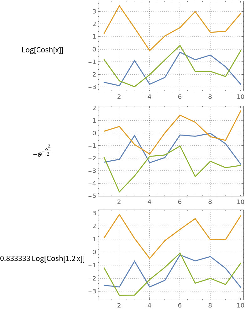 |
Note that we used a small number of steps in order to obtain similar but different results. Using a sufficiently large number of steps (say, 20) we get almost the same results (with the matrix mat).
Here are signal generating functions:
| In[19]:= | ![Clear[s1, s2, s3]
s1[t_] := Sin[600 \[Pi] t/10000 + 6*Cos[120 \[Pi] t/10000]] + 1.2
s2[t_] := Sin[\[Pi] t/10] + 1.2
s3[t_?NumericQ] := (((QuotientRemainder[t, 23][[2]] - 11)/9)^5 + 2.8)/
2 + 0.2](https://www.wolframcloud.com/obj/resourcesystem/images/c3f/c3fea6ef-e925-4a13-832e-bc1ebe467c12/07c77428e2301078.png) |
Here is a mixing matrix:
| In[20]:= |
Form a matrix of the signals:
| In[21]:= | ![nSize = 600;
S = Table[{s1[t], s2[t], s3[t]}, {t, 0, nSize, 0.5}];
Dimensions[S]](https://www.wolframcloud.com/obj/resourcesystem/images/c3f/c3fea6ef-e925-4a13-832e-bc1ebe467c12/5a7197332055c410.png) |
| Out[21]= |
Plot the values:
| In[22]:= |
| Out[22]= | 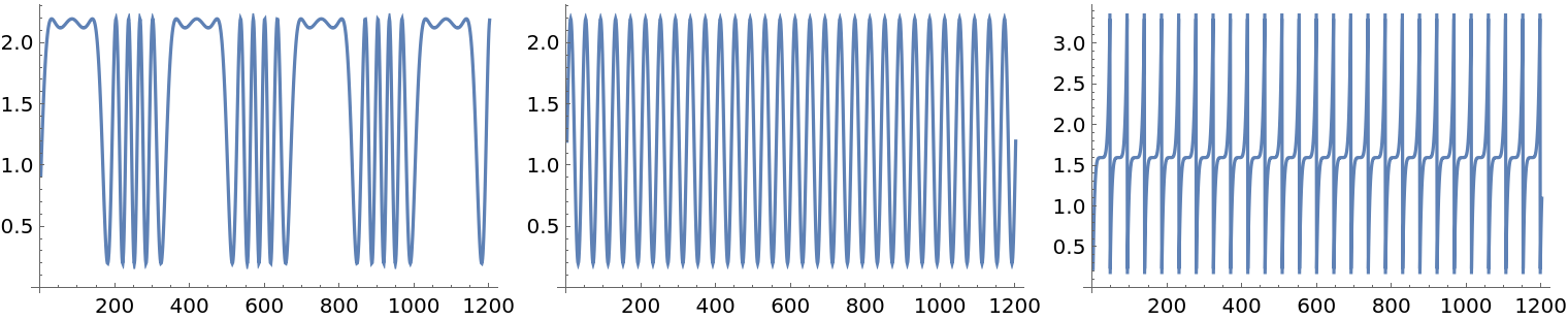 |
Create and plot the mixed signals matrix:
| In[23]:= |
| Out[23]= | 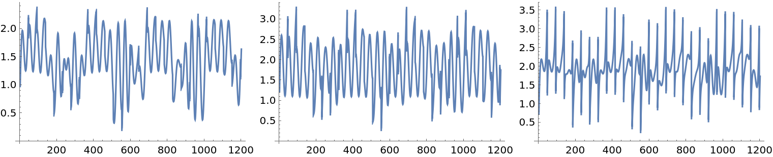 |
Find the ICA decomposition:
| In[24]:= |
Approximation norm:
| In[25]:= |
| Out[25]= |
Visualize the ICA-identified source signals:
| In[26]:= |
| Out[26]= | 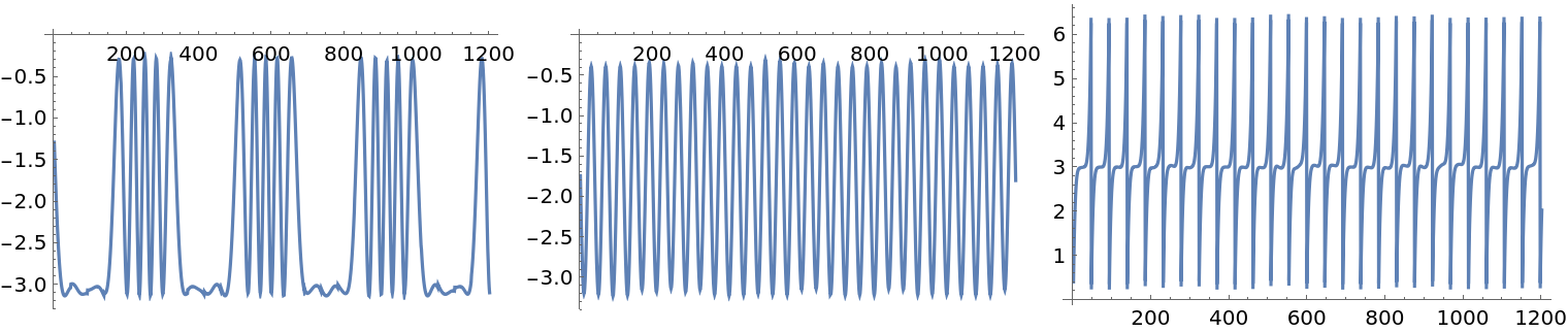 |
The ICA computations can be sensitive to the presence of outliers. Here we add a small number of outliers to the original mixed signals:
| In[27]:= | ![M1 = M + RandomChoice[{0.005, 0.995} -> {1, 0}, Dimensions[M]];
MapThread[
ListLinePlot[{##}, PlotLegends -> {"with outliers", "original"}] &, {Transpose[M1], Transpose[M]}]](https://www.wolframcloud.com/obj/resourcesystem/images/c3f/c3fea6ef-e925-4a13-832e-bc1ebe467c12/44d39678d2808b5a.png) |
| Out[27]= | 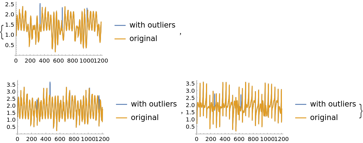 |
Here we apply ICA to the new mixed signals:
| In[28]:= |
We see that the found components are not that good compared to the components found for the original mixed signals data:
| In[29]:= |
| Out[29]= | 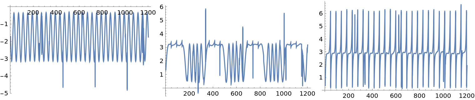 |
This work is licensed under a Creative Commons Attribution 4.0 International License