Wolfram Function Repository
Instant-use add-on functions for the Wolfram Language
Function Repository Resource:
Simple tool for working with regions of interest on images
ResourceFunction["ImageROIConvert"][roi] represents a rectangular region of interest roi, given by<|"x"→xmin,"y"→ymin,"w"→width,"h"→height|>. | |
ResourceFunction["ImageROIConvert"][roi,image,transform] represents a rectangular region of interest roi in an image after applying a coordinate system transform. | |
ResourceFunction["ImageROIConvert"][roi, {width,height}, transform] represents a rectangular region of interest roi in an image of given dimensions after applying a coordinate system transform. |
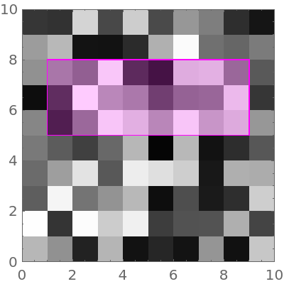
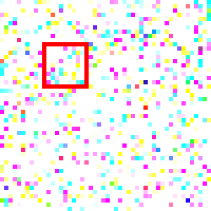
Sometimes ROIs (regions of interest) are provided in terms of width and height:
| In[1]:= |
![img = RandomImage[1, {10, 10}, ImageSize -> 200];
HighlightImage[img, ResourceFunction[
"ImageROIConvert"][<|"x" -> 1, "y" -> 5, "w" -> 8, "h" -> 3|>], Frame -> True]](https://www.wolframcloud.com/obj/resourcesystem/images/f86/f86a4536-c387-4c6a-979a-e313b1bc85e2/133050047d5f7605.png)
|
| Out[2]= |
|
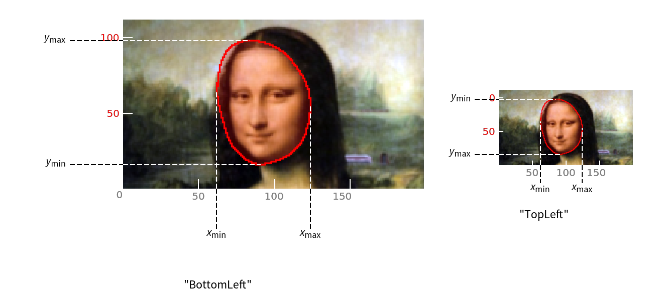
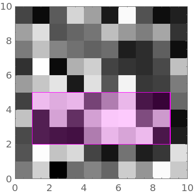
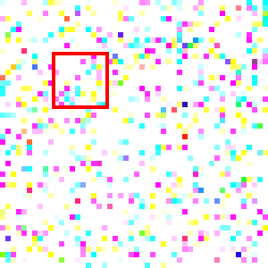
Having to switch between coordinate systems with a top or bottom origin is a very common. When converting to a "TopLeft" or "BottomRight" origin, you need to supply the original image (or its dimensions):
| In[3]:= |
![HighlightImage[img, ResourceFunction[
"ImageROIConvert"][<|"x" -> 1, "y" -> 5, "w" -> 8, "h" -> 3|>, img, "TopLeft"], Frame -> True]](https://www.wolframcloud.com/obj/resourcesystem/images/f86/f86a4536-c387-4c6a-979a-e313b1bc85e2/4dcc595c34aacc08.png)
|
| Out[3]= |
|
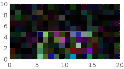
As a convenience, ImageROIConvert handles regions given in XYWH form. They can be given as real pixel coordinate values in the range [0,w]⨯[0,h] or as scaled coordinates in the range [0,1]⨯[0,1]:
| In[4]:= |
![img = RandomImage[1, {20, 10}, ImageSize -> 200, ColorSpace -> "CMYK"];
rect = <|"x" -> .25, "y" -> 0, "w" -> .5, "h" -> .5|>;
HighlightImage[img, ResourceFunction["ImageROIConvert"][rect, img, "BottomLeft", "ScaledCoordinates" -> True], "Darken", Frame -> True]](https://www.wolframcloud.com/obj/resourcesystem/images/f86/f86a4536-c387-4c6a-979a-e313b1bc85e2/71d7e23e6d54ba27.png)
|
| Out[4]= |
|
To run this example, you first need to connect to a python executable in an environment (e.g. here my environment is named dl) where both opencv and pyzmq are installed (for more details see this workflow):
| In[5]:= |
![$sess = StartExternalSession[{"Python", "Executable" -> "/Users/msollami/anaconda3/envs/dl/bin/python"}]](https://www.wolframcloud.com/obj/resourcesystem/images/f86/f86a4536-c387-4c6a-979a-e313b1bc85e2/1e07ee14d75d9481.png)
|
| Out[5]= |
|
Now let's draw a rectangle on an image with the python computer vision library OpenCV (which is named cv2 in code):
| In[6]:= |
![img = RandomImage[10, {50, 50}, ColorSpace -> "RGB"];
ExternalEvaluate[$sess, "imgD=" <> ExportString[ImageData[img, "Byte"], "PythonExpression"]]
Image[ExternalEvaluate[$sess, "import numpy as np; import cv2 as cv;
img = np.asarray(imgD, np.uint8);
cv.rectangle(img, (10, 10), (20, 20), (255, 0, 0), 1);
img"], ImageSize -> 150]](https://www.wolframcloud.com/obj/resourcesystem/images/f86/f86a4536-c387-4c6a-979a-e313b1bc85e2/45dc3829bbc98b34.png)
|
| Out[7]= |
|
Convert the coordinate system's origin to "BottomLeft" to plot it:
| In[8]:= |
![HighlightImage[img, {EdgeForm[{Thick, Red}], FaceForm[None], ResourceFunction["ImageROIConvert"][Rectangle[{10, 10}, {20, 20}], img, "BottomLeft"]}, ImageSize -> 150]](https://www.wolframcloud.com/obj/resourcesystem/images/f86/f86a4536-c387-4c6a-979a-e313b1bc85e2/091452f3fd7742d3.png)
|
| Out[8]= |
|
Create a Rectangle region of interest and highlight it:
| In[9]:= |
![img = ConstantImage[0, {20, 20}, ImageSize -> 150];
rect = Rectangle[{3, 5}, {10, 15}];
HighlightImage[img, {White, EdgeForm[Thickness[.05]], FaceForm[None], rect}]](https://www.wolframcloud.com/obj/resourcesystem/images/f86/f86a4536-c387-4c6a-979a-e313b1bc85e2/48a4e96e4a90f659.png)
|
| Out[10]= |

|
To use this in OpenCV (whose python library is named cv2), we ask for a "TopLeft" origin coordinate transform:
| In[11]:= |
|
| Out[11]= |
|
Now we can send it to a session for drawing (requires a python installation):
| In[12]:= |
![ExternalEvaluate[$sess, "[[x1,y1], [x2,y2]]=" <> ExportString[List @@ converted, "PythonExpression"]];
Image[ExternalEvaluate[$sess, "import numpy as np; import cv2 as cv;
img = np.zeros((20, 20, 3), np.uint8);
cv.rectangle(img, (x1, y1), (x2, y2), (255, 255, 255), 1);
img"], ImageSize -> 150]](https://www.wolframcloud.com/obj/resourcesystem/images/f86/f86a4536-c387-4c6a-979a-e313b1bc85e2/5b7ef02ab28636e8.png)
|
| Out[13]= |

|
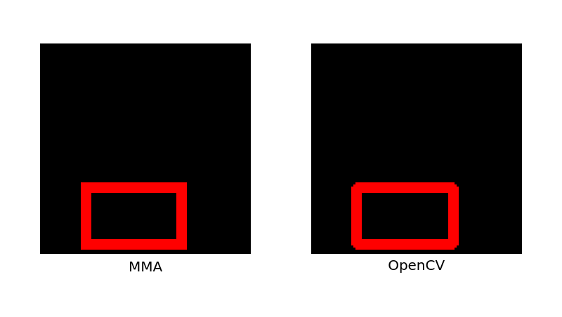
Create a Rectangle with scaled coordinates for use in OpenCV (this example requires a python installation):
| In[14]:= |
![img = ConstantImage[0, {100, 100}, ImageSize -> 150];
rect = Rectangle[RandomReal[1, 2], RandomReal[1, 2]]; (* scaled coordinates *)
pyrect = List @@ ResourceFunction["ImageROIConvert"][rect, img, "TopLeft", "ScaledCoordinates" -> True];
ExternalEvaluate[$sess, "[[x1,y1], [x2,y2]]=" <> ExportString[pyrect, "PythonExpression"]];
GraphicsRow[{Labeled[
HighlightImage[
img, {Red, EdgeForm[Thickness[.05]], FaceForm[None], ResourceFunction["ImageROIConvert"][rect, img, "ScaledCoordinates" -> True]}], "MMA"], Labeled[Image[
ExternalEvaluate[$sess, "import numpy as np; import cv2 as cv;
img = np.zeros((100, 100, 3), np.uint8);
cv.rectangle(img, (x1, y1), (x2, y2), (255, 0, 0), 3);
img"], ImageSize -> 150], "OpenCV"]}, ImageSize -> 400]](https://www.wolframcloud.com/obj/resourcesystem/images/f86/f86a4536-c387-4c6a-979a-e313b1bc85e2/52236f2b2f4a2557.png)
|
| Out[18]= |
|
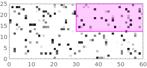
If setting the option "ScaledCoordinates"→True, the coordinates of the input are assumed to lie between zero and one:
| In[19]:= |
![rect = Rectangle[{.5, .5}, {1, 1}];
HighlightImage[img = RandomImage[10, {60, 25}, ImageSize -> 250], ResourceFunction["ImageROIConvert"][rect, img, "ScaledCoordinates" -> True], Frame -> True]](https://www.wolframcloud.com/obj/resourcesystem/images/f86/f86a4536-c387-4c6a-979a-e313b1bc85e2/487866f2a5056dbb.png)
|
| Out[20]= |
|
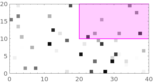
| In[21]:= |
![rect = <|"x" -> .5, "y" -> .5, "w" -> .5, "h" -> .5|>;
HighlightImage[img = RandomImage[20, {40, 20}, ImageSize -> 250], ResourceFunction["ImageROIConvert"][rect, img, "BottomRight", "ScaledCoordinates" -> True], Frame -> True]](https://www.wolframcloud.com/obj/resourcesystem/images/f86/f86a4536-c387-4c6a-979a-e313b1bc85e2/3caa024a8e692d56.png)
|
| Out[22]= |
|
Convert object detections from the Wolfram Language to Python (this example requires a python installation):
| In[23]:= |
![(* Evaluate this cell to get the example input *) CloudGet["https://www.wolframcloud.com/obj/0ae6ad10-8f60-4c16-877b-fccdab51f058"]](https://www.wolframcloud.com/obj/resourcesystem/images/f86/f86a4536-c387-4c6a-979a-e313b1bc85e2/65c71ba8655fdebe.png)
|
| In[24]:= |
|
| Out[24]= |
|
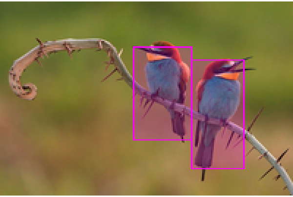
Highlight the identified bounding boxes:
| In[25]:= |
|
| Out[25]= |
|
Convert the bird's bounding boxes to have top left origin:
| In[26]:= |
|
| Out[26]= |
|
Export the variables to the python session:
| In[27]:= |
|
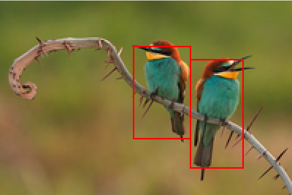
Draw the boxes:
| In[28]:= |
![Image[ExternalEvaluate[$sess, "import numpy as np; import cv2 as cv;
img = np.asarray(imgData, np.uint8);
birds = np.asarray(birds, np.uint8);
for b in birds:
cv.rectangle(img, tuple(b[0]), tuple(b[1]), (255, 0, 0), 1);
img"], ImageSize -> 300]](https://www.wolframcloud.com/obj/resourcesystem/images/f86/f86a4536-c387-4c6a-979a-e313b1bc85e2/02fde62378209063.png)
|
| Out[28]= |
|
This work is licensed under a Creative Commons Attribution 4.0 International License