Function Repository Resource:

HyperellipticODE

Get a physicist's constructive proof of Fuchs's theorem on hyperelliptic curves

Contributed by: Bradley Klee

ResourceFunction["HyperellipticODE"][V,{p,q, α}]

returns the ODE constraining integral periods T(α) associated with a Hamiltonian constraint of the form α=2H(p,q)=p²+2V(q), and V(q) a non-linear q-polynomial.

ResourceFunction["HyperellipticODE"][V,{p,q,α},certificate]

also returns a checked and checkable Association containing proof data, when certificate is set to True.

Details

The acronym ODE stands for "Ordinary Differential Equation".

Specification of variables {p, q, α} is optional if the potential is written in terms of the formal variable q.

For our purposes, a rational, elliptic or hyperelliptic level curve may be written in set-builder notation as:

𝒞(α)={(p,q)∈ℂ²:α=2H(p,q)=p²+2V(q):V(q)=∑n=1Nv_nqⁿ :v_n∈ℝ }

Also, at least one v_n with n>1 must not equal to zero.

When viewed in four dimensional space, such a level curve is really a level surface with measurable genus.

Whether the curve is rational, elliptic, or hyperelliptic depends on the degree cutoff N as well as particular values of the v_n.

ResourceFunction["HyperellipticODE"] does not distinguish between harmonic, elliptic, or hyperelliptic curves.

ResourceFunction["HyperellipticODE"] cannot accept linear potentials as input because linear potentials do not admit periodic solutions.

Time t is defined in terms of the tangents D_t{p, q}={-∂_qH,∂_pH}.

The invariant time differential may then be written most directly as dt=dq/p.

Subsequent α-derivatives of the integrand dt are written as

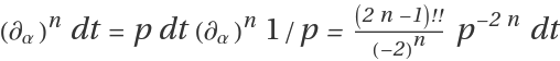
The primary task of ResourceFunction["HyperellipticODE"] is to compute a set of coefficients c_n(α) and a certificate Ξ(q, p) such that:

When this condition is satisfied, the exact differential can be integrated to zero around a contour, which implies:

This is the form of the minimal output, an ordinary differential equation constraining period functions T(α).

The proof data described above can be put into an Association:

Potential

Hamiltonian

α = 2H

Coordinates

{p, q,α}

Tangents

{-∂_qH,∂_pH}

Time Forms

(∂_α)ⁿdt,n=0, 1, …

ODE Coefficients

c_n,n=0, 1, …

Certificate Function

Truth Value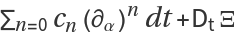

The last item with Key "Truth Value" should auto-evaluate to 0 for valid data.

For more details refer to "An Update on the Computational Theory of Hamiltonian Period Functions", especially Chapter 3.

Examples

Basic Examples (5)

Find the period ODE coefficients of an elliptic curve:

In[1]:=

$TraditionalForm[ ResourceFunction[ "HyperellipticODE"][(1/2) (\[FormalQ]^2 - Sqrt[4/27] \[FormalQ]^3)]]$

Out[1]=

Solve the ODE to find the real-valued hypergeometric period function:

In[2]:=

$With[{Hyper2F1pars = First[ Solve[# == 0 & /@ Flatten[CoefficientList[ ResourceFunction[ "HyperellipticODE"][(1/2) (\[FormalQ]^2 - Sqrt[4/27] \[FormalQ]^3), True]["ODE Coefficients"] - {-a b, c - (a + b + 1) \[FormalAlpha], \[FormalAlpha] (1 - \[FormalAlpha])} k, \[FormalAlpha]]]]]}, TraditionalForm[\[FormalCapitalT][\[FormalAlpha]] == 2 Pi Hypergeometric2F1[a, b, c, \[FormalAlpha]] /. Hyper2F1pars]]$

Out[2]=

Display the proof data in a table:

In[3]:=

$Grid[Transpose[{Text /@ Keys[#], TraditionalForm /@ Values[#]}], Frame -> All, FrameStyle -> Lighter@Gray, Spacings -> {5, 1} ] &@ResourceFunction[ "HyperellipticODE"][(1/2) (\[FormalQ]^2 - Sqrt[4/27] \[FormalQ]^3), True]$

Out[3]=

Write and check an unusual proof that the harmonic oscillator has a constant period:

In[4]:=

$Grid[Transpose[{Text /@ Keys[#], TraditionalForm /@ Values[#]}], Frame -> All, FrameStyle -> Lighter@Gray, Spacings -> {5, 1} ] &@ResourceFunction["HyperellipticODE"][(1/2) \[FormalQ]^2, True]$

Out[4]=

Continue on to a random hyperelliptic curve with terms up to q⁶:

In[5]:=

$Construct[#["Potential"] -> #["Truth Value"] &, ResourceFunction["HyperellipticODE"][ Dot[\[FormalQ]^Range[6], RandomInteger[{-5, 5}, 6]], True]]$

Out[5]=

Scope (2)

Potentials can be specified with undetermined coefficients:

In[6]:=

$CoefficientList[ ResourceFunction[ "HyperellipticODE"][(1/2) (\[FormalQ]^2 - \[FormalQ]^3 + b \[FormalQ]^4), True]["ODE Coefficients"], \[FormalAlpha], 6] // TableForm$

Out[6]=

This sort of data leads quite readily to finding interesting cases:

In[7]:=

$With[{ODEcs = ResourceFunction["HyperellipticODE"][ (1/2) (\[FormalQ]^2 - \[FormalQ]^3 + (3/8) \[FormalQ]^4), True]["ODE Coefficients"]}, Association["ODE Coefficients" -> ODEcs, "Well Integrable" -> Expand[D[ODEcs[[-1]], \[FormalAlpha]] - ODEcs[[2]]], "Solution Space" -> T[\[FormalAlpha]] /. First[DSolve[Dot[ ODEcs, D[T[\[FormalAlpha]], {\[FormalAlpha], #}] & /@ {0, 1, 2} ] == 0, T[\[FormalAlpha]], \[FormalAlpha] ]]]]$

Out[7]=

Properties and Relations (1)

Proof data is dynamically checkable in a short time:

In[8]:=

$AnnihilationCondition[ potential_, vars_, dtForms_, ODEcs_, cert_ ] := Expand[Expand[Times[Plus[ Dot[D[cert, #] & /@ vars[[1 ;; 2]], {D[-potential, vars[[2]]], vars[[1]]}], Dot[ODEcs, dtForms ]], vars[[1]]^(2 Length[ODEcs] - 2)] ] /. vars[[1]] -> Sqrt[vars[[3]] - 2 potential]]$

In[9]:=

$With[{proof = ResourceFunction["HyperellipticODE"][ (1/2) (\[FormalQ]^2 - Sqrt[4/27] \[FormalQ]^3), True]}, AnnihilationCondition[ proof["Potential"], proof["Coordinates"], proof["Time Forms"], proof["ODE Coefficients"], proof["Certificate Function"]]]$