Wolfram Function Repository
Instant-use add-on functions for the Wolfram Language
Function Repository Resource:
Measure the linear-drift-insensitive, two-sample, phase/frequency stability
ResourceFunction["HadamardDeviation"][data,r,taus] calculates the linear-drift insensitive two-sample deviation of data along sample times taus at rate r. |
| {{n}} | attempts to place n logarithmic spaced samples |
| d | places logarithmic spaced samplings with log base d |
| {τ1,τ2,…} | tries to use the specified sample times |
| All | uses all possible sample times |
| Automatic | tries to place a reasonable amount of samples along the whole possible time range |
Calculating the Hadamard deviation for a small sample set at a rate of 2 samples per time unit:
| In[1]:= |
| Out[1]= |
Display overlapping Hadamard deviation of white noise at a rate of 0.1 for automatically chosen sampling points:
| In[2]:= | ![data = RandomFunction[WhiteNoiseProcess[1], {100}]["Values"];
hdev = ResourceFunction["HadamardDeviation"][data, 0.1, Automatic];
ListLogLogPlot[hdev, FrameLabel -> {"Averaging time \[Tau]", "Hadamard Deviation \!\(\*SubscriptBox[\(\[Sigma]\), \(y\)]\)"}, IntervalMarkersStyle -> Gray]](https://www.wolframcloud.com/obj/resourcesystem/images/8c2/8c2df5bb-d77b-4d3a-901e-ffa47ed1bc14/34ddd1d9c57e995b.png) |
| Out[4]= | 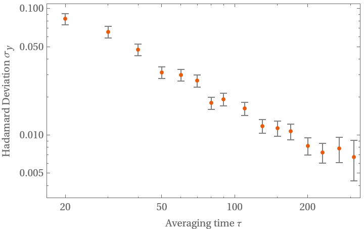 |
Display overlapping Hadamard deviation of white noise at a rate of 0.1 for certain sampling points:
| In[5]:= | ![data = RandomFunction[WhiteNoiseProcess[1], {200}]["Values"];
hdev = ResourceFunction["HadamardDeviation"][data, 0.1, {20, 50, 100, 200, 400}];
ListLogLogPlot[hdev, GridLines -> Automatic]](https://www.wolframcloud.com/obj/resourcesystem/images/8c2/8c2df5bb-d77b-4d3a-901e-ffa47ed1bc14/5ef43f68f7cf2edd.png) |
| Out[6]= | 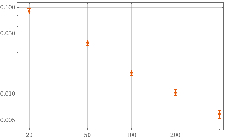 |
Sample at all possible times:
| In[7]:= | ![data = RandomFunction[WhiteNoiseProcess[1], {100}]["Values"];
hdev = ResourceFunction["HadamardDeviation"][data, 1, All];
ListLogLogPlot[hdev]](https://www.wolframcloud.com/obj/resourcesystem/images/8c2/8c2df5bb-d77b-4d3a-901e-ffa47ed1bc14/6f8aacd4d89bb3d0.png) |
| Out[8]= | 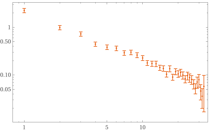 |
Try to sample at 4 different time values:
| In[9]:= | ![data = RandomFunction[WhiteNoiseProcess[1], {200}]["Values"];
hdev = ResourceFunction["HadamardDeviation"][data, 1, {{4}}];
ListLogLogPlot[hdev]](https://www.wolframcloud.com/obj/resourcesystem/images/8c2/8c2df5bb-d77b-4d3a-901e-ffa47ed1bc14/1acca46de91e796e.png) |
| Out[11]= | 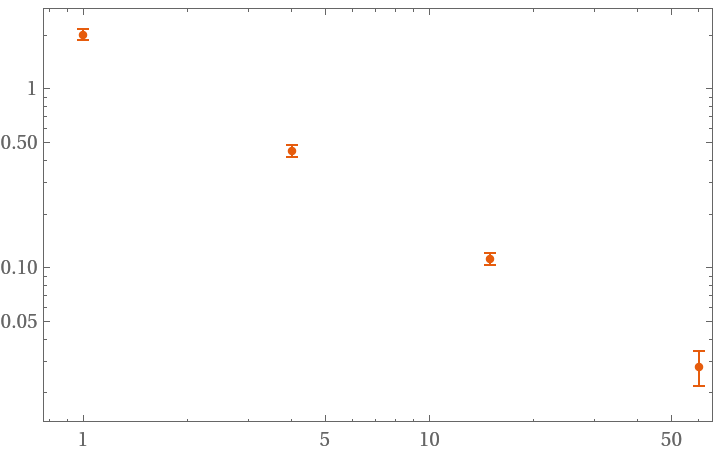 |
The function will try to use a fast evaluation method when the data array is fully real and otherwise prints a warning:
| In[12]:= | ![data = RandomFunction[WhiteNoiseProcess[1], {100}]["Values"];
hdev = ResourceFunction["HadamardDeviation"][data~Join~{Pi}, 1, Automatic];
ListLogLogPlot[hdev]](https://www.wolframcloud.com/obj/resourcesystem/images/8c2/8c2df5bb-d77b-4d3a-901e-ffa47ed1bc14/5a1f5292ceee5daf.png) |
| Out[14]= | 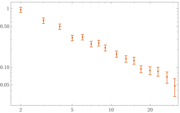 |
FrequencyData accepts a Boolean as argument. True signals the use of frequency data as opposed to phase data:
| In[15]:= | ![data = RandomFunction[WhiteNoiseProcess[1], {100}]["Values"];
hdev = ResourceFunction["HadamardDeviation"][data, 1, All, "FrequencyData" -> True];
ListLogLogPlot[hdev]](https://www.wolframcloud.com/obj/resourcesystem/images/8c2/8c2df5bb-d77b-4d3a-901e-ffa47ed1bc14/4035e27b9868a84c.png) |
| Out[17]= | 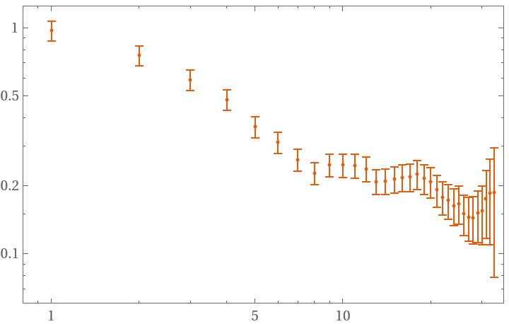 |
Overlapping accepts a Boolean as argument. False signals the use of non overlapping strides in the deviation sampling:
| In[18]:= | ![data = RandomFunction[WhiteNoiseProcess[1], {100}]["Values"];
hdev = ResourceFunction["HadamardDeviation"][data, 1, All, "Overlapping" -> False];
ListLogLogPlot[hdev]](https://www.wolframcloud.com/obj/resourcesystem/images/8c2/8c2df5bb-d77b-4d3a-901e-ffa47ed1bc14/0254a457ecee1fe7.png) |
| Out[19]= | 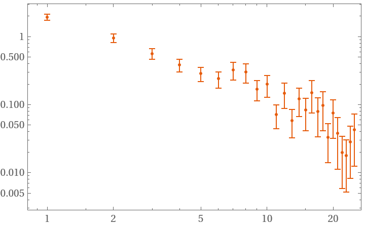 |
Distinguish random walk from white noise by their distinct slope:
| In[20]:= | ![datas = N[
RandomFunction[#, {10000}]["Values"]] & /@ {WhiteNoiseProcess[], RandomWalkProcess[0.5]};
hdevs = ResourceFunction["HadamardDeviation"][#, 1, Automatic] & /@ datas;
ListLogLogPlot[hdevs]](https://www.wolframcloud.com/obj/resourcesystem/images/8c2/8c2df5bb-d77b-4d3a-901e-ffa47ed1bc14/747005c30388f51b.png) |
| Out[22]= | 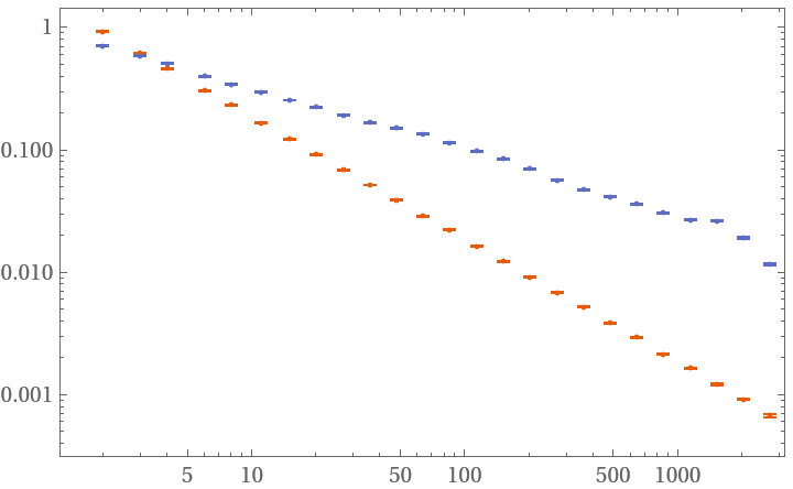 |
The Hadamard deviation is is approximately equal to the Allan deviation except for linear drifts:
| In[23]:= | ![data = RandomFunction[WhiteNoiseProcess[], {10000}]["Values"] + Accumulate[ConstantArray[10^-3, 10001]];
hdev = ResourceFunction["HadamardDeviation"][data, 1.0, Automatic, "FrequencyData" -> True];
adev = ResourceFunction["AllanDeviation"][data, 1.0, Automatic, "FrequencyData" -> True];
ListLogLogPlot[{hdev, adev}, PlotLegends -> {"Hadamard deviation", "Allan deviation"}]](https://www.wolframcloud.com/obj/resourcesystem/images/8c2/8c2df5bb-d77b-4d3a-901e-ffa47ed1bc14/24d9835fd1868acb.png) |
| Out[24]= | 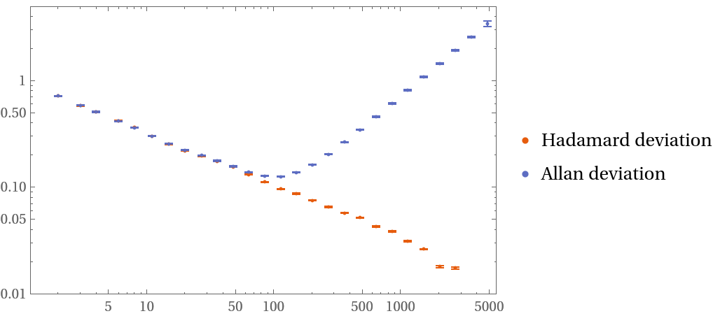 |
Using the fast algorithm is approximately 2 times faster:
| In[25]:= |
| Out[26]= |
| In[27]:= |
| Out[27]= |
Requesting a certain amount of samples will not necessarily result in this amount of deviations:
| In[28]:= |
| Out[29]= |
This work is licensed under a Creative Commons Attribution 4.0 International License