Details
ResourceFunction["GridSampleLayer"] is a lookup operator to a feature array using pixel coordinates. Inside a neural network this can be used to warp features between two views or to project a higher-order tensor by looking up pixel positions. This layer is often necessary in tasks where the coordinate array is a learning objective such as optical flow or when a feature array is a learning objective such as learnable parametric encodings for NERF or DeepSDF.
ResourceFunction["GridSampleLayer"] is typically used inside
NetChain,
NetGraph, etc.
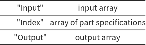
The output of
ResourceFunction["GridSampleLayer"] is a
NetGraph with the following ports:
The possible values for mode of ResourceFunction["GridSampleLayer"] are:
The "Input" is a 2D feature array of dimensions {n,inWidth,inHeight}.
The "Index" is a 2D index array of dimensions {2,outWidth,outHeight}.
In ResourceFunction["GridSampleLayer"][n,{inWidth,inHeight},{outWidth,outHeight}], the arguments are defined as follows:
Bilinear interpolation is a sampling technique where the output at a point is the weighted average of the four nearest points on the grid. This sampling is the same as in
ResizeLayer with the "linear"
Resampling method, i.e. piecewise linear interpolation.
This GridSampleLayer is an implementation of torch.nn.functional.grid_sample (spatial 4-D) with this specific set of parameters:
-mode= 'bilinear'
-padding_mode= 'reflection'
-align_corners=False

![coords = Transpose[Table[{i, j}, {i, 1, 16}, {j, 1, 16}], {2, 3, 1}];
sample = gsLayer[<|"Input" -> array, "Index" -> coords|>];
Image[sample, Interleaving -> False, ImageSize -> Small]](https://www.wolframcloud.com/obj/resourcesystem/images/751/75141204-da2d-47c5-a0ee-e5742371fe65/60ea303a534da923.png)

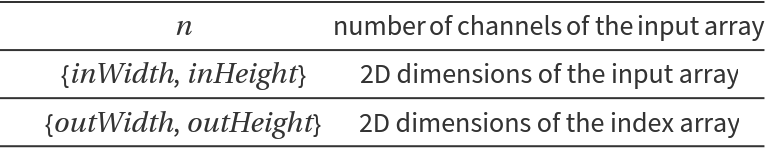
![Manipulate[(
coords = Transpose[Table[{i + g, j + h}, {i, 1, 16}, {j, 1, 16}], {2, 3, 1}];
sample = gsLayer[<|"Input" -> array, "Index" -> coords|>];
Image[sample, Interleaving -> False, ImageSize -> Small]
), {{g, 6}, 0, 12, 0.5}, {{h, 6}, 0, 12, 0.5}]](https://www.wolframcloud.com/obj/resourcesystem/images/751/75141204-da2d-47c5-a0ee-e5742371fe65/4f4d15617923ba08.png)
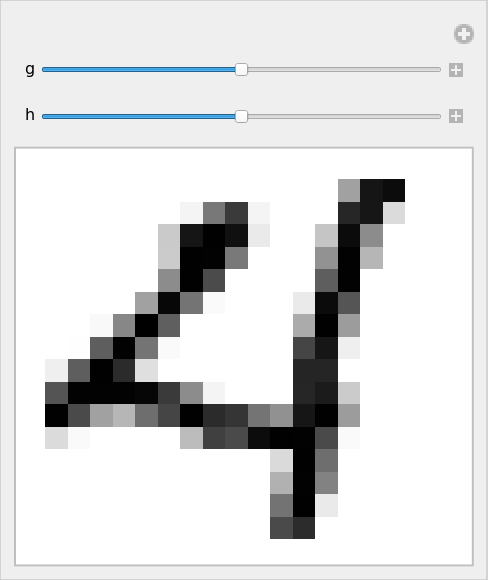
![Manipulate[(
coords = Transpose[
Table[{i, j}, {i, g - 7/s, g + 8/s, 1/s}, {j, h - 7/s, h + 8/s, 1/s}], {2, 3, 1}];
sample = gsLayer[<|"Input" -> array, "Index" -> coords|>];
Image[sample, Interleaving -> False, ImageSize -> Small]
), {{g, 14}, 8, 20, 1}, {{h, 14}, 8, 20, 1}, {{s, 1}, 1, 4, 0.1}]](https://www.wolframcloud.com/obj/resourcesystem/images/751/75141204-da2d-47c5-a0ee-e5742371fe65/1e365ca0986798b5.png)
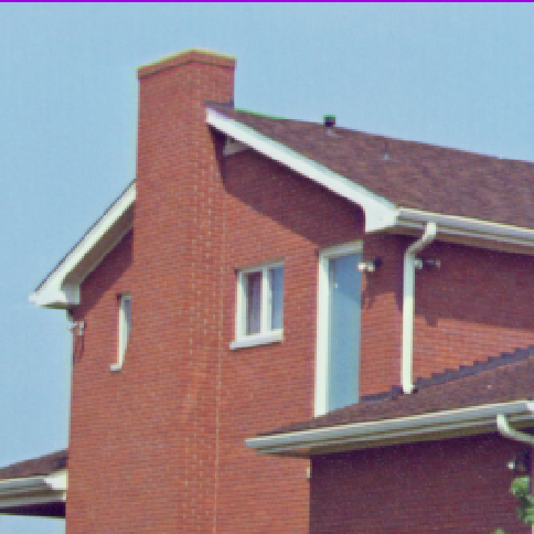
![image = ExampleData[{"TestImage", "House"}]
input = ImageData[image, Interleaving -> False];
{n, inH, inW} = Dimensions[input];](https://www.wolframcloud.com/obj/resourcesystem/images/751/75141204-da2d-47c5-a0ee-e5742371fe65/52ca2908faa23257.png)
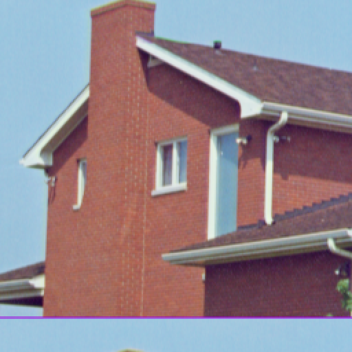
![t = 0.2;
coords = Transpose[
Table[{i, j}, {i, -1 + t, 1 + t, 2/(inH - 1)}, {j, -1, 1, 2/(inW - 1)}], {2, 3, 1}];
im = gsHouseLayer[<|"Input" -> input, "Index" -> coords|>];
Image[im, Interleaving -> False]](https://www.wolframcloud.com/obj/resourcesystem/images/751/75141204-da2d-47c5-a0ee-e5742371fe65/70136c1e159c0874.png)
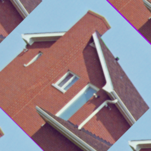
![\[Theta] = Pi/4;
coords = coords = Transpose[
Table[{{Cos[\[Theta]], -Sin[\[Theta]]}, {Sin[\[Theta]], Cos[\[Theta]]}} . {i, j}, {i, -1, 1, 2/(inH - 1)}, {j, -1, 1, 2/(inW - 1)}], {2, 3, 1}];
im = gsHouseLayer[<|"Input" -> input, "Index" -> coords|>];
Image[im, Interleaving -> False]](https://www.wolframcloud.com/obj/resourcesystem/images/751/75141204-da2d-47c5-a0ee-e5742371fe65/0187b9d2d40531b9.png)
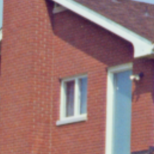
![{{c0x, c0y}, {c1x, c1y}} = {{64, 64}, {192, 192}};
lx = Rescale[c0x, {1, inH}, {-1, 1}];
hx = Rescale[c1x, {1, inH}, {-1, 1}];
ly = Rescale[c0y, {1, inW}, {-1, 1}];
hy = Rescale[c1y, {1, inW}, {-1, 1}];
coords = coords = Transpose[
Table[{i, j}, {i, lx, hx, (hx - lx)/(inH - 1)}, {j, ly, hy, (hy - ly)/(inW - 1)}], {2, 3, 1}];
im = gsHouseLayer[<|"Input" -> input, "Index" -> coords|>];
Image[im, Interleaving -> False]](https://www.wolframcloud.com/obj/resourcesystem/images/751/75141204-da2d-47c5-a0ee-e5742371fe65/72147cb9d987edef.png)
![parametricGrid = NetInitialize@NetGraph@FunctionLayer[Block[{array, sample}, (
array = NetArrayLayer["Output" -> {16, 48, 64}][];
sample = ResourceFunction["GridSampleLayer"][16, {48, 64}, {32, 32}, "Coordinates"][<|"Input" -> array, "Index" -> #Input|>]
)] &]](https://www.wolframcloud.com/obj/resourcesystem/images/751/75141204-da2d-47c5-a0ee-e5742371fe65/3e75af57f28f5473.png)
![indices = Transpose[Table[{i, j}, {i, 9, 40}, {j, 17, 48}], {2, 3, 1}];
sample = parametricGrid[indices];
sample // Dimensions](https://www.wolframcloud.com/obj/resourcesystem/images/751/75141204-da2d-47c5-a0ee-e5742371fe65/5b1f42e04de55c4a.png)
![(* Evaluate this cell to get the example input *) CloudGet["https://www.wolframcloud.com/obj/1d30c4b3-508f-447d-b6d9-02bc79b5a205"]](https://www.wolframcloud.com/obj/resourcesystem/images/751/75141204-da2d-47c5-a0ee-e5742371fe65/1afbc5aec7f2e59c.png)
![f[pt_] := With[{s = {.5, .5}}, Module[{r, a},
r = Sqrt[Norm[pt - s] Max[s]]; a = ArcTan @@ (pt - s);
s + r {Cos[a], Sin[a]}]];
coords = Transpose[
Table[f[{i, j}]*2 - 1, {i, 0, 1, 1/(inH - 1)}, {j, 0, 1, 1/(inW - 1)}], {2, 3, 1}];
out = gsDistortionLayer[<|"Input" -> input, "Index" -> coords|>];
Image[out, Interleaving -> False]](https://www.wolframcloud.com/obj/resourcesystem/images/751/75141204-da2d-47c5-a0ee-e5742371fe65/7d4b9dc911dfa4c2.png)

![f[pt_] := With[{s = {0.55, 0.55}}, Module[{r, a},
r = Norm[pt - s]^2/Norm[s]; a = ArcTan @@ (pt - s);
s + r {Cos[a], Sin[a]}]]
coords = Transpose[
Table[f[{i, j}]*2 - 1, {i, 0, 1, 1/(inH - 1)}, {j, 0, 1, 1/(inW - 1)}], {2, 3, 1}];
out = gsDistortionLayer[<|"Input" -> input, "Index" -> coords|>];
Image[out, Interleaving -> False]](https://www.wolframcloud.com/obj/resourcesystem/images/751/75141204-da2d-47c5-a0ee-e5742371fe65/211071a308386134.png)
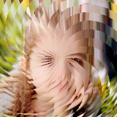
![f[pt_] := With[{s = {.5, .5}}, Module[{r, a},
r = Norm[pt - s]^2/Max[s]; a = ArcTan @@ (pt - s)/Pi*180;
pt + {Mod[(a/200 + r/2.), 16/200.] - 8/200., 0}]]
coords = Transpose[
Table[f[{i, j}]*2 - 1, {i, 0, 1, 1/(inH - 1)}, {j, 0, 1, 1/(inW - 1)}], {2, 3, 1}];
out = gsDistortionLayer[<|"Input" -> input, "Index" -> coords|>];
Image[out, Interleaving -> False]](https://www.wolframcloud.com/obj/resourcesystem/images/751/75141204-da2d-47c5-a0ee-e5742371fe65/2e29eb59162c3469.png)
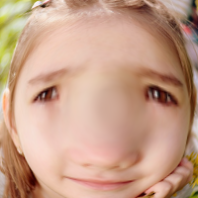
![Clear[f];
f[pt_] := With[{s = {.5, .5}}, Module[{r, a, an},
r = Norm[pt - s]; a = ArcTan @@ (pt - s); an = a + 2 r;
s + r {Cos[an], Sin[an]}]];
coords = Transpose[
Table[f[{i, j}]*2 - 1, {i, 0, 1, 1/(inH - 1)}, {j, 0, 1, 1/(inW - 1)}], {2, 3, 1}];
out = gsDistortionLayer[<|"Input" -> input, "Index" -> coords|>];
Image[out, Interleaving -> False]](https://www.wolframcloud.com/obj/resourcesystem/images/751/75141204-da2d-47c5-a0ee-e5742371fe65/5c458456ff0b2792.png)

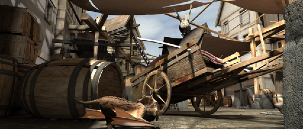
![(* Evaluate this cell to get the example input *) CloudGet["https://www.wolframcloud.com/obj/e27c1a7b-4bdd-4614-ad08-7e30dc9e6f44"]](https://www.wolframcloud.com/obj/resourcesystem/images/751/75141204-da2d-47c5-a0ee-e5742371fe65/4a4d8929b09a08da.png)
![(* Evaluate this cell to get the example input *) CloudGet["https://www.wolframcloud.com/obj/a33e081c-cf45-4340-a51d-e0c949225b51"]](https://www.wolframcloud.com/obj/resourcesystem/images/751/75141204-da2d-47c5-a0ee-e5742371fe65/439e560ea3c79372.png)
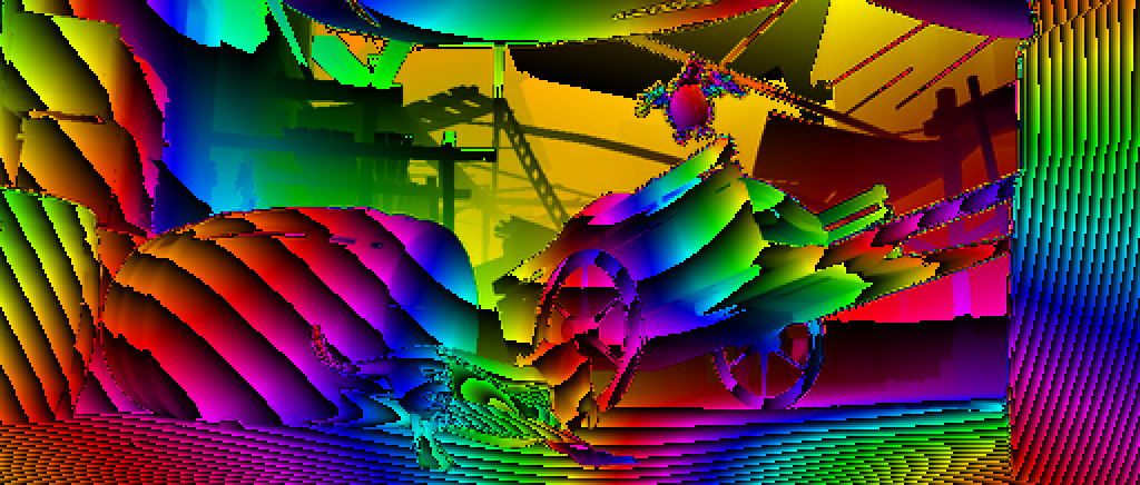
![out = Table[
gsOpticalFlow[<|"Input" -> input, "Index" -> coords + k*Reverse[flo]|>, TargetDevice -> "GPU"], {k,
0, 1, 0.1}];
frames = Image[#, Interleaving -> False] & /@ Reverse[out];
FrameListVideo[Join[frames, Reverse[frames]]]](https://www.wolframcloud.com/obj/resourcesystem/images/751/75141204-da2d-47c5-a0ee-e5742371fe65/28b6a501c54857e0.png)