Wolfram Function Repository
Instant-use add-on functions for the Wolfram Language
Function Repository Resource:
Get a version of 3D graphics with segments replaced by tubes
ResourceFunction["Graphics3DWireFrame"][graphics3D] gives a version of graphics3D with segments replaced by tubes. |
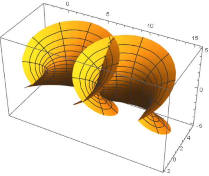
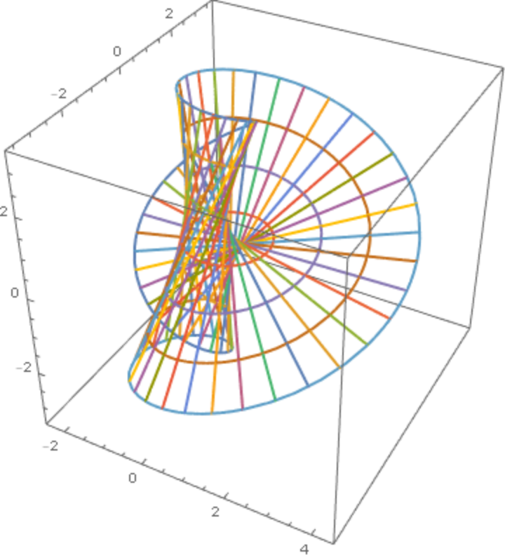
A surface:
| In[1]:= |
![catalan[a_][t_][u_, v_] := {(a Cos[t]) (u - Cosh[v] Sin[u]) + (a Sin[t]) (v - Cos[u] Sinh[v]), (a Cos[t]) (1 - Cos[u] Cosh[v]) + ((a Sin[t]) Sin[u]) Sinh[
v], ((4 a) (1 - Cos[u/2] Cosh[v/2])) Sin[
t] - (((4 a) Cos[t]) Sin[u/2]) Sinh[v/2]}](https://www.wolframcloud.com/obj/resourcesystem/images/7a7/7a7d6205-1cb4-48aa-862d-f021b4d9db2d/7a29a0715e339410.png)
|
Plot the surface:
| In[2]:= |
|
| Out[2]= |
|
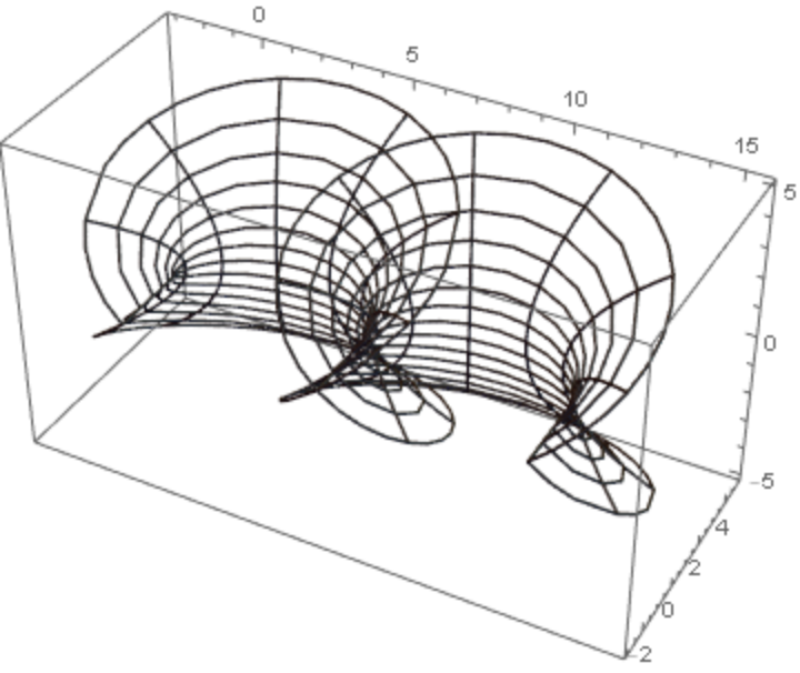
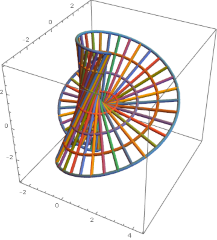
Another wire frame with a standard mesh:
| In[3]:= |
|
| Out[3]= |
|
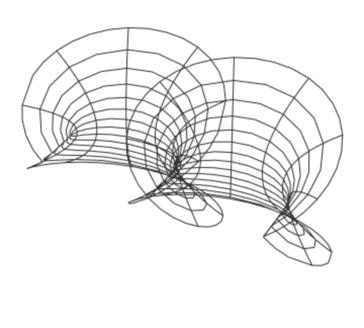
A similar appearance using PlotStyle:
| In[4]:= |
|
| Out[4]= |
|
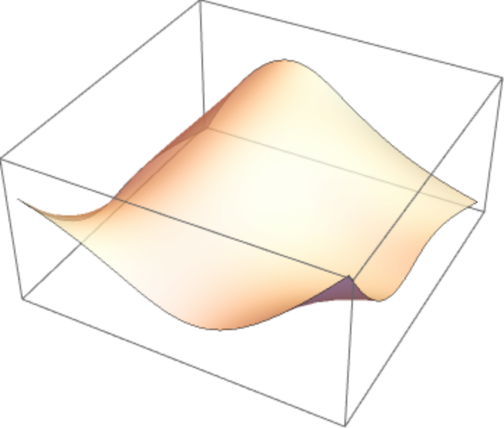
Another surface:
| In[5]:= |
|
| Out[5]= |
|
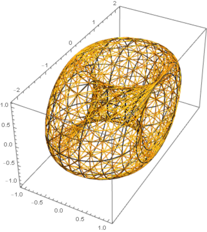
A Möbius strip made of curves:
| In[6]:= |
![f[u_, v_] := {(1 + u Cos[v/2]) Cos[v], (1 + u Cos[v/2]) Sin[v], u Sin[v/2]}; Show[
ParametricPlot3D[
Evaluate@Table[ f[u, i], {i, -\[Pi], \[Pi], 1/6}], {u, -\[Pi], \[Pi]}, PlotRange -> All],
ParametricPlot3D[
Evaluate@Table[
f[j, v], {j, -\[Pi], \[Pi], \[Pi]/3}], {v, -\[Pi], \[Pi]}]]](https://www.wolframcloud.com/obj/resourcesystem/images/7a7/7a7d6205-1cb4-48aa-862d-f021b4d9db2d/4a5d57e8d2af3235.png)
|
| Out[6]= |
|
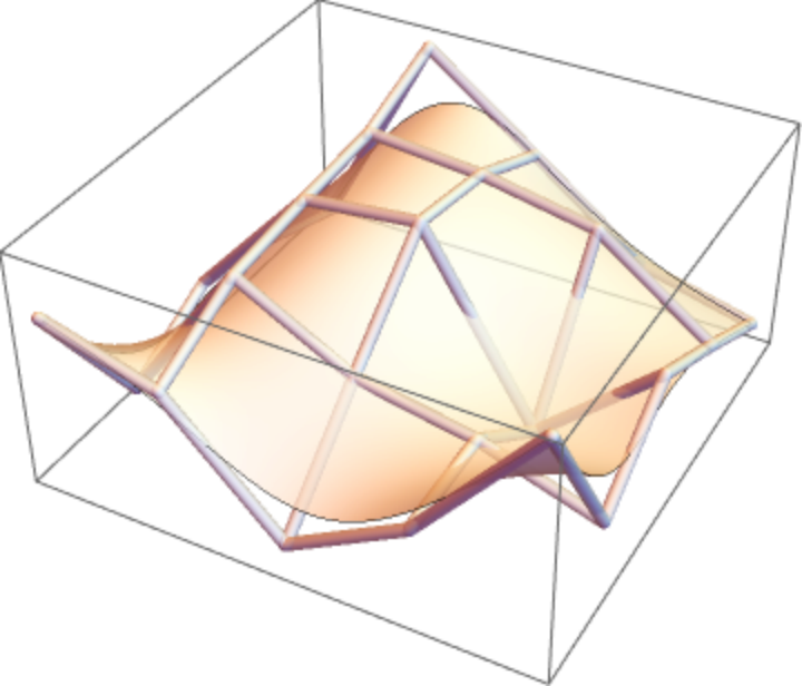
Plot the wire frame:
| In[7]:= |
|
| Out[7]= |
|
A B–spline surface:
| In[8]:= |
|
| In[9]:= |
|
| Out[9]= |
|
| In[10]:= |
|
| Out[10]= |
|
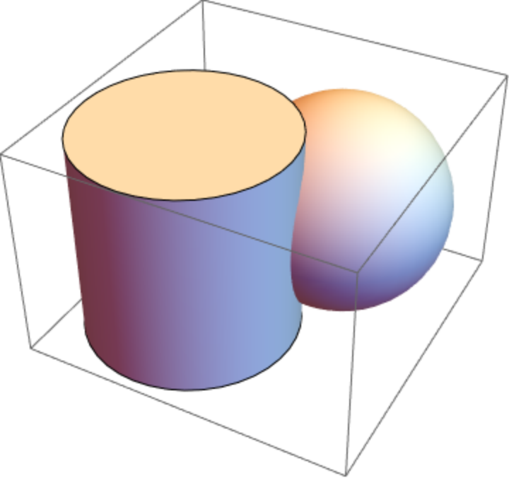
Take a region:
| In[11]:= |
|
| Out[11]= |
|
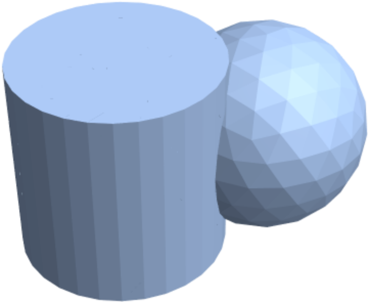
Extract the primitives:
| In[12]:= |
|
| Out[12]= |
|
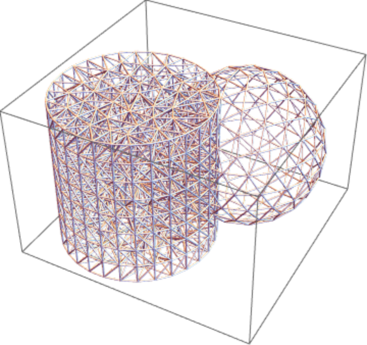
Make the wire frame:
| In[13]:= |
|
| Out[13]= |
|
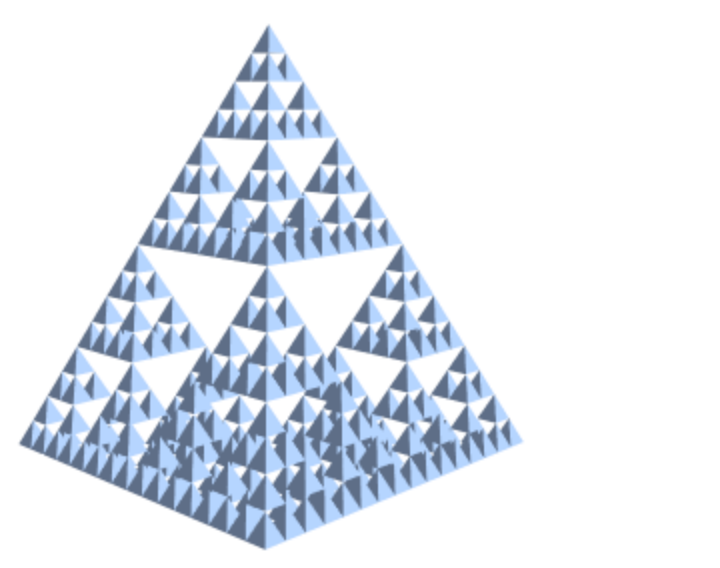
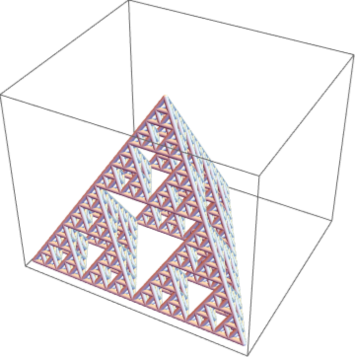
A fractal region:
| In[14]:= |
|
| Out[14]= |
|
| In[15]:= |
|
| Out[15]= |
|
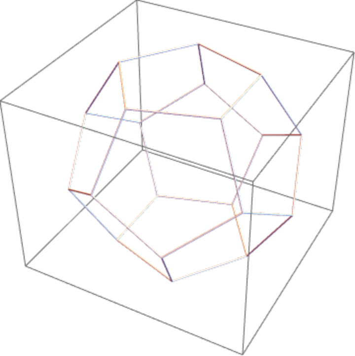
Show a dodecahedron:
| In[16]:= |
|
Show a dodecahedron:
| In[17]:= |
|
| Out[17]= |
|
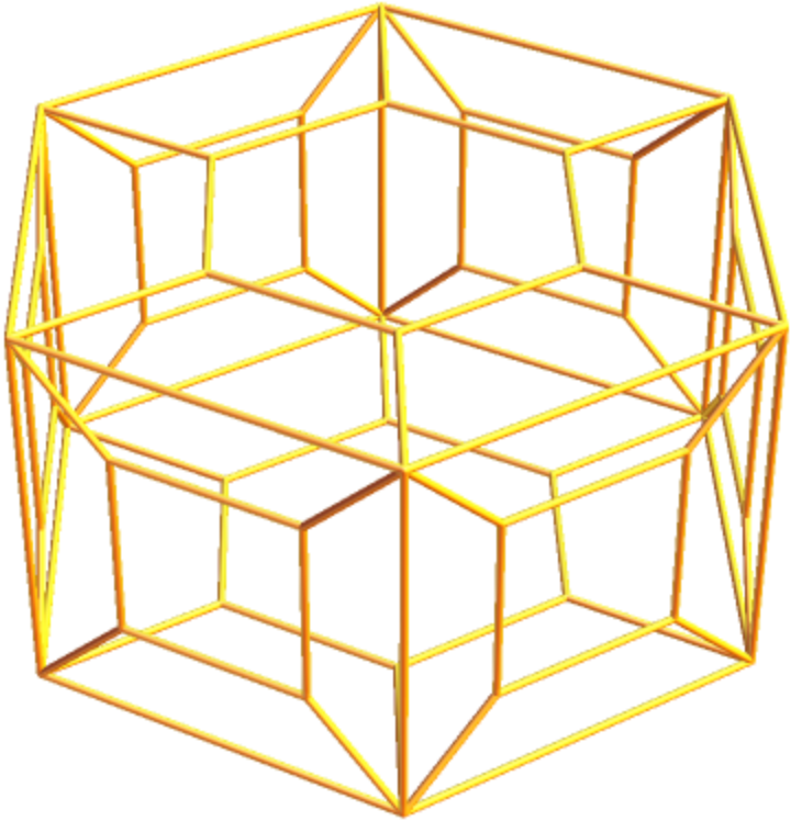
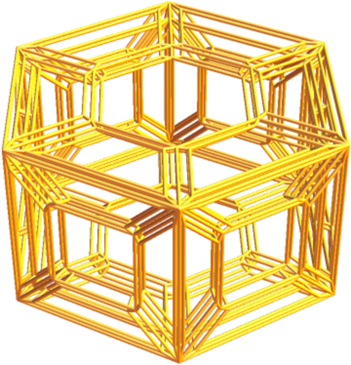
Show a hexagonal prism:
| In[18]:= |
![uehp = ResourceFunction["PerforatePolygons"][
Entity["Polyhedron", {"Prism", 6}]["Graphics3D"]]](https://www.wolframcloud.com/obj/resourcesystem/images/7a7/7a7d6205-1cb4-48aa-862d-f021b4d9db2d/79bff4308962f3df.png)
|
| Out[18]= |

|
| In[19]:= |
|
| Out[19]= |
|
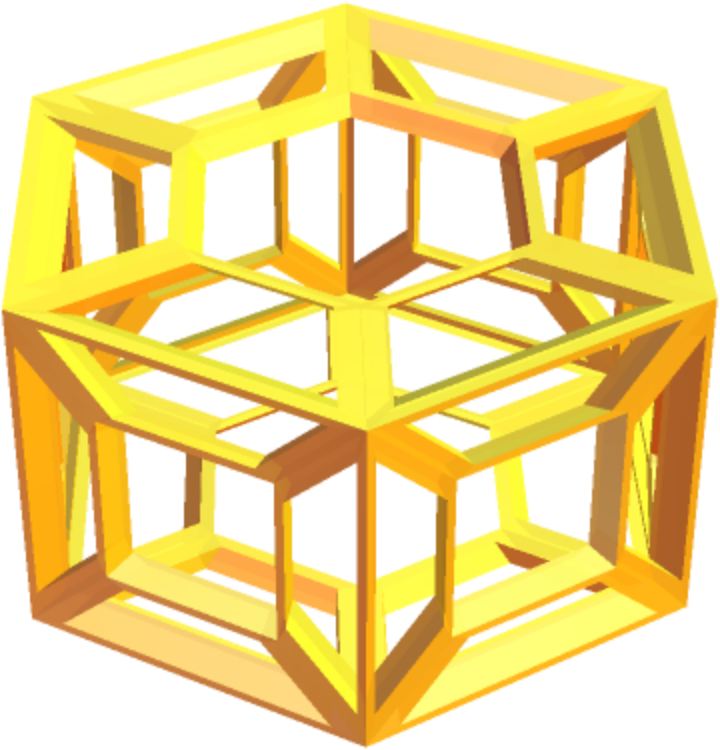
Outline the prism:
| In[20]:= |
|
| Out[20]= |
|
Show a dodecahedron:
| In[21]:= |
|
| Out[21]= |
|
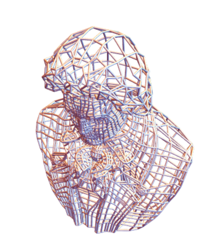
A 3D model:
| In[22]:= |
|
| Out[22]= |
|
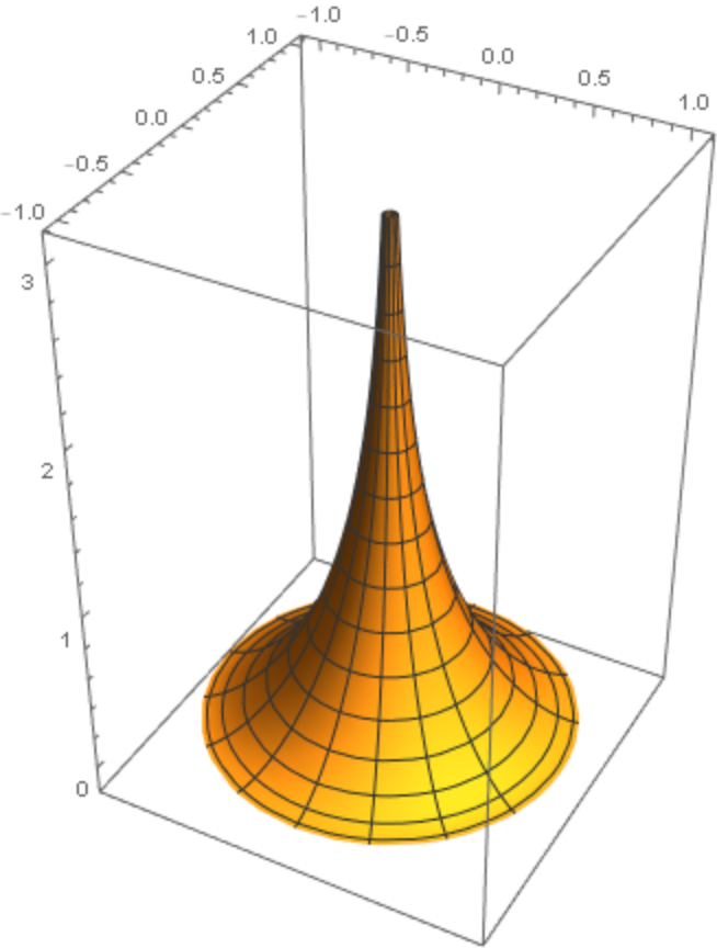
A surface:
| In[23]:= |
|
| Out[23]= |
|
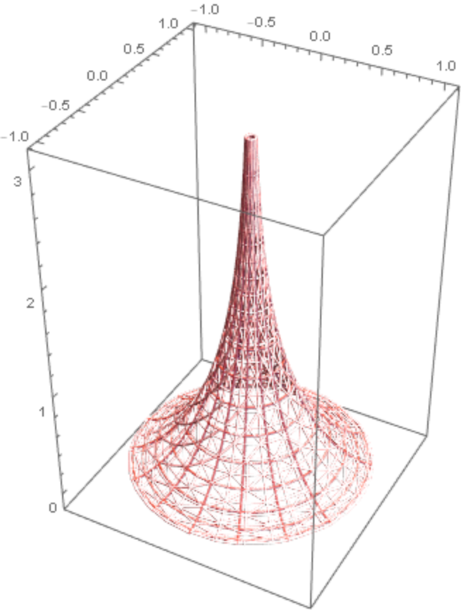
Change style of the wire frame:
| In[24]:= |
|
| Out[24]= |
|
This work is licensed under a Creative Commons Attribution 4.0 International License