Basic Examples (2)
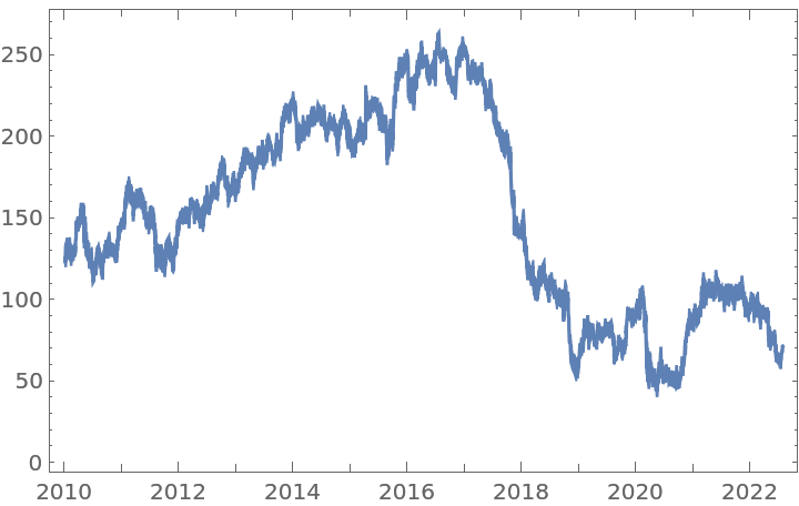
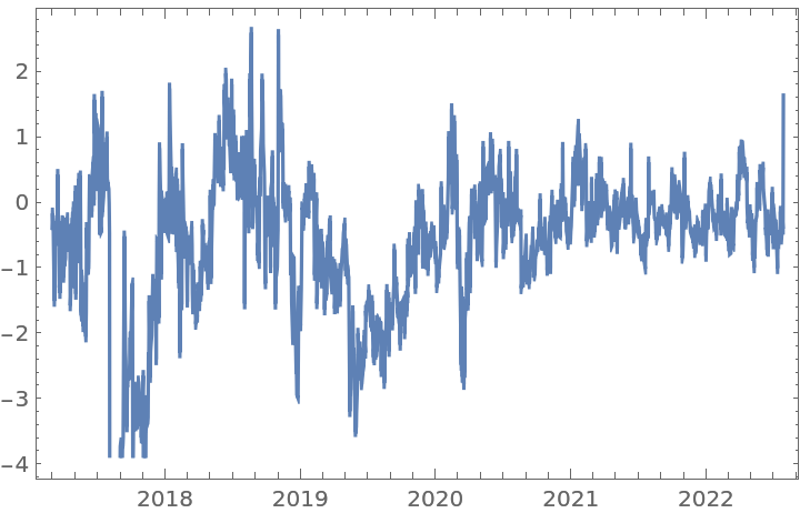
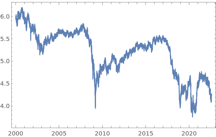
Get a time series of closing prices and visualize it:
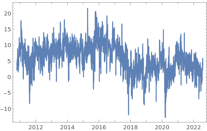
Compute the half difference of the time series and visualize it:
Scope (2)
Get a time series of closing prices:
With order 1, FractionalDTimeSeries gives the usual first difference:
However, applying the half-difference twice on the original time series yields an equivalent first difference, but with fewer data points and on a slightly different scale:
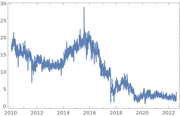
Get a time series of closing prices:
Apply a fractional difference of order 0.3531 to the original time series with the default tolerance:
For the same time series, a fractional difference of order 0.3531 and a larger tolerance will generate a time series with more data points:
In contrast, a fractional difference of the same order 0.3531, but with a smaller tolerance, will generate a time series with fewer data points:
Applications (3)
Simulate an ARIMAProcess with linear trend and apply a fractional difference of order 0.5:
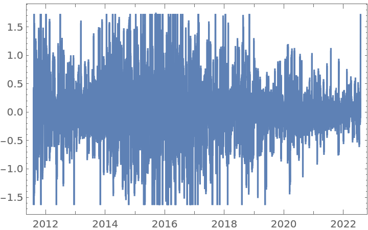
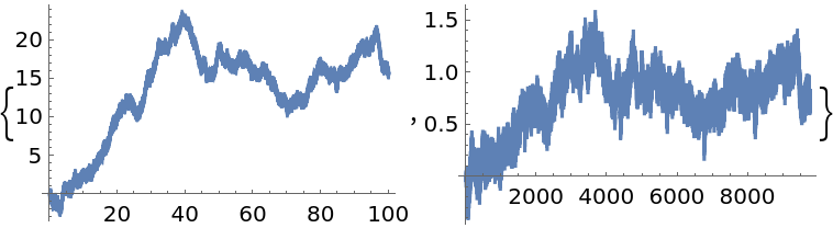
Simulate an FractionalBrownianMotionProcess with Hurst index 0.65 and apply a fractional difference of order 0.45 to it:
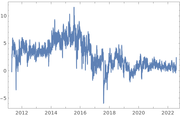
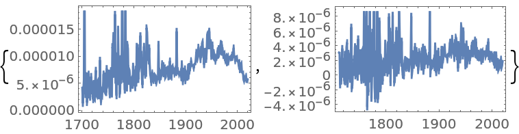
Get a time series of the frequencies of the word "Peru" in typical published text, and apply a fractional difference of order 0.35 and a tolerance of 0.01 to it:
Possible Issues (4)
FractionalDTimeSeries requires the order to be a positive real number. Negative orders (integration) are currently not implemented:
FractionalDTimeSeries requires the tolerance to be positive:
If the tolerance is too small, no transformation will be performed:
If the tolerance is set too high, the transformed time series will be essentially the same as the original one, but in a different scale:
Neat Examples (4)
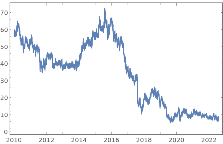
A logarithmically-transformed time series:
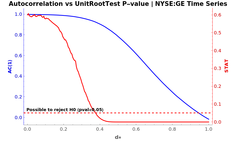
Find the relationship between the statistical value of a UnitRootTest and the CorrelationFunction of a transformed time series, by using several orders between 0 and 1:
Apply a UnitRootTest (red axis) on each differentiated time series to see up from which level of d is possible to reject H0. Also, compute its CorrelationFunction at lag 1 (blue axis) to compare:
Plot the results:
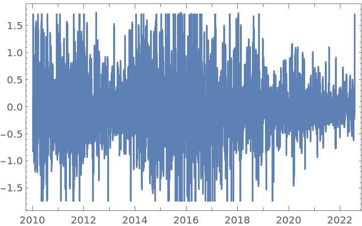
![BlockRandom[SeedRandom[170]; sample = RandomFunction[ARIMAProcess[{-0.1}, 1, {0.2}, 0.1], {1, 1*^4}]];
{ListLinePlot[sample], ListLinePlot[
ResourceFunction["FractionalDTimeSeries"][sample, 0.5]["Values"]]}](https://www.wolframcloud.com/obj/resourcesystem/images/ede/ede9645e-0120-4755-aa41-23f5a7b2521d/6cee0e842ca86009.png)
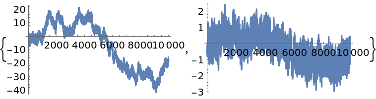
![BlockRandom[SeedRandom[150]; sample = RandomFunction[
FractionalBrownianMotionProcess[0.65], {0, 100, 0.01}]];
{ListLinePlot[sample], ListLinePlot[
ResourceFunction["FractionalDTimeSeries"][sample, 0.45]["Values"]]}](https://www.wolframcloud.com/obj/resourcesystem/images/ede/ede9645e-0120-4755-aa41-23f5a7b2521d/3a5d66977475eb2e.png)
![sample = WordFrequencyData["Peru", "TimeSeries"];
{DateListPlot[sample], DateListPlot[
ResourceFunction["FractionalDTimeSeries"][sample, 0.35, 0.01]]}](https://www.wolframcloud.com/obj/resourcesystem/images/ede/ede9645e-0120-4755-aa41-23f5a7b2521d/0ae5e148855e5ec3.png)
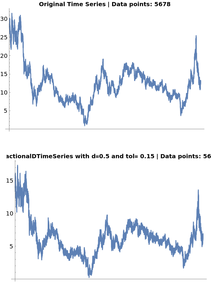
![ts = FinancialData["F", "Close", "Jan. 1, 2000"];
fdshightol = ResourceFunction["FractionalDTimeSeries"][ts, 0.5, 0.15]](https://www.wolframcloud.com/obj/resourcesystem/images/ede/ede9645e-0120-4755-aa41-23f5a7b2521d/0683cafcec691e92.png)
![Row[
{ListLinePlot[ts, ImageSize -> 350, PlotLabel -> Style["Original Time Series | Data points: " <> ToString@(Length@(ts["Values"])), Darker@Black, 10, Bold]], ListLinePlot[fdshightol, ImageSize -> 350, PlotLabel -> Style["FractionalDTimeSeries with d=0.5 and tol= 0.15 | Data points: " <> ToString@(Length@(fdshightol["Values"])),
Darker@Black, 10, Bold]]}]](https://www.wolframcloud.com/obj/resourcesystem/images/ede/ede9645e-0120-4755-aa41-23f5a7b2521d/5e5e3f0d05e32fc9.png)
![baseDs = Range[0, 1, 0.005];
setFSeries = Table[{d, ResourceFunction["FractionalDTimeSeries"][ts, d]}, {d, baseDs}];](https://www.wolframcloud.com/obj/resourcesystem/images/ede/ede9645e-0120-4755-aa41-23f5a7b2521d/59eb15febc72a653.png)
![corrPlot = ListLinePlot[
{#[[1]], #[[2]]} & /@ statACFDataPlot, ImagePadding -> {{50, 50}, {45, 2}},
PlotStyle -> Blue, Frame -> {True, True, False, False},
FrameStyle -> {Automatic, Blue, Automatic, Automatic}, FrameTicks -> {None, All, None, None},
PlotLabel -> Style["Autocorrelation vs UnitRootTest P-value | NYSE:GE Time Series", Black, 13, Bold],
FrameLabel -> {{Style["AC(1)", Bold], None}, {Style["d*", 11, Bold], None}},
ImageSize -> 500];
statPlot = ListLinePlot[
{#[[1]], #[[3]]} & /@ statACFDataPlot, ImagePadding -> {{50, 50}, {45, 2}},
PlotStyle -> Red,
Frame -> {False, False, False, True},
FrameTicks -> {{None, All}, {None, None}},
FrameStyle -> {Automatic, Automatic, Automatic, Red},
FrameLabel -> {{None, Style["STAT", Bold]}, {None, None}},
PlotLabel -> Style[" "],
ImageSize -> 500,
GridLines -> {None, {0.05}},
GridLinesStyle -> Directive[AbsoluteThickness[3/2], Red, Dashed],
Epilog -> {Text[
Style["Possible to reject H0 (pval<0.05)", 9, Bold], Scaled[{0.015, 0.125}], {-1, 0}]}
];](https://www.wolframcloud.com/obj/resourcesystem/images/ede/ede9645e-0120-4755-aa41-23f5a7b2521d/5b9071ea4e431fa3.png)