Wolfram Function Repository
Instant-use add-on functions for the Wolfram Language
Function Repository Resource:
Compute the finite difference stencil for a specified set of variables and their derivatives
ResourceFunction["FiniteDifferenceStencil"][deriv,vars,depvar,indepvar] returns the finite difference stencil associated with the derivative expression deriv in terms of the specified variables vars and the order of the finite difference approximation. |
| "Stencil" | finite difference stencil |
| "Coefficients" | coefficients of the stencil |
| "Order" | order of the approximation |
Find the finite difference stencil for the first derivative spanning three points:
| In[1]:= |
| Out[1]= |
Find the finite difference stencil for a second derivative spanning three points:
| In[2]:= |
| Out[2]= |
Find the finite difference stencil for a second derivative spanning three one-sided points:
| In[3]:= |
| Out[3]= |
Find the finite difference stencil for a third derivative spanning five points:
| In[4]:= |
| Out[4]= |  |
Use functions and their derivatives to obtain high order finite difference approximation with same stencil size:
| In[5]:= |
| Out[5]= |  |
Use the order of the finite difference stencil to obtain optimal stencil positions:
| In[6]:= |
| Out[6]= |  |
Solve for the arbitrary parameter to obtain the optimal stencil position for the first derivative:
| In[7]:= |
| Out[7]= |
The order of the finite difference approximation can be increased by choosing the appropriate parameters:
| In[8]:= |
| Out[8]= |  |
| In[9]:= | ![With[{a = -Sqrt[3/5]}, ResourceFunction["FiniteDifferenceStencil"][
f''[x], {f[x - dx], f[x], f[x + dx], f'[x - a dx], f'[x]}, f, x]]](https://www.wolframcloud.com/obj/resourcesystem/images/5e7/5e781cd2-a1b8-49a6-b730-92d3884266fb/6783dc4e1613432e.png) |
| Out[9]= |  |
Derivative values can be computed from function values using finite difference approximation. Generate the data:
| In[10]:= |
Use a three point finite difference coefficients to get a second order approximation of the first derivative:
| In[11]:= | ![dx = x[[2]] - x[[1]];
coeffs = ResourceFunction["FiniteDifferenceStencil"][
f'[s], {f[s - dx], f[s], f[s + dx]}, f, s]["Coefficients"];
Short[firstDeriv = Partition[fval, 3, 1] . coeffs, 3]](https://www.wolframcloud.com/obj/resourcesystem/images/5e7/5e781cd2-a1b8-49a6-b730-92d3884266fb/40f8f159739d5b4a.png) |
| Out[12]= |
Compare the results with the reference values:
| In[13]:= |
| Out[13]= | 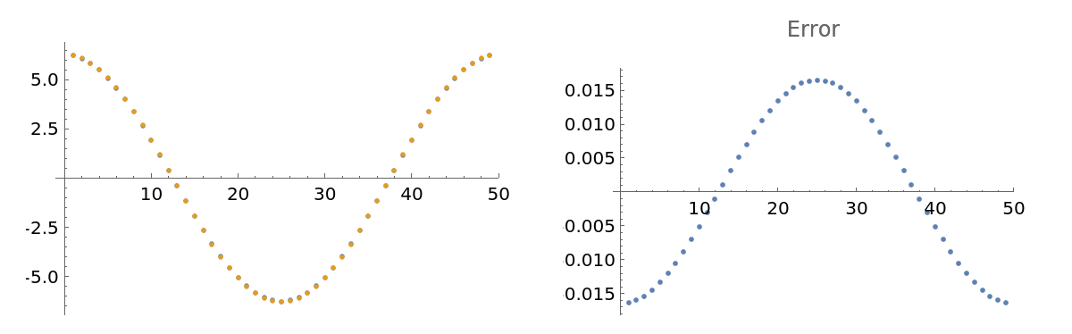 |
The error can be reduced by using more data points:
| In[14]:= | ![coeffs = ResourceFunction["FiniteDifferenceStencil"][
f'[s], {f[s - 2 dx], f[s - dx], f[s], f[s + dx], f[s + 2 dx]}, f, s]["Coefficients"];
Short[firstDeriv2 = Partition[fval, 5, 1] . coeffs, 3]](https://www.wolframcloud.com/obj/resourcesystem/images/5e7/5e781cd2-a1b8-49a6-b730-92d3884266fb/20a79bc375e710a3.png) |
| Out[15]= |
Plot the error associated with the better approximation:
| In[16]:= |
| Out[16]= | 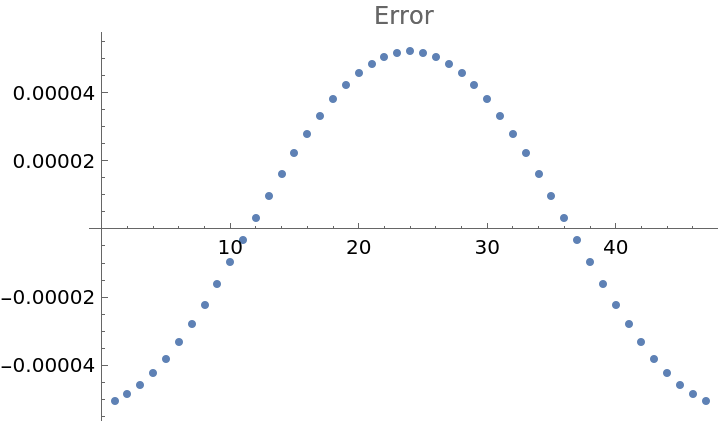 |
Generate finite difference stencils for complex grid points:
| In[17]:= | ![vars = Flatten[Table[f[x + i*h + j*I*h], {i, -1, 1}, {j, -1, 1}]];
Table[res = ResourceFunction["FiniteDifferenceStencil"][D[f[x], {x, i}], vars, f, x];
{MatrixForm[Partition[res["Coefficients"], 3]], res["Order"]}, {i, 4}] // Column](https://www.wolframcloud.com/obj/resourcesystem/images/5e7/5e781cd2-a1b8-49a6-b730-92d3884266fb/078b63cf7dcaa106.png) |
| Out[18]= |  |
The complex stencils are able to generate high accuracy approximations. Approximate the third derivative of a function at a specific point:
| In[19]:= | ![fun[x_] := Sin[2 Pi x];
cgrid[x_] := Flatten[Table[x + i*h + j*I*h, {i, -1, 1}, {j, -1, 1}]];
coeffs = ResourceFunction["FiniteDifferenceStencil"][D[f[x], {x, 3}], vars, f, x]["Coefficients"]](https://www.wolframcloud.com/obj/resourcesystem/images/5e7/5e781cd2-a1b8-49a6-b730-92d3884266fb/0634d34c4c8f1caa.png) |
| Out[20]= |
Approximate the third derivative at x=0.1 for various spacing h:
| In[21]:= |
| Out[21]= | 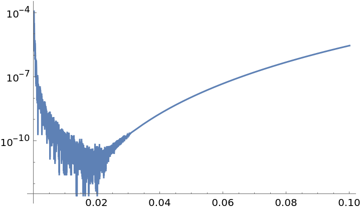 |
Convert the finite difference stencils into differentiation matrices:
| In[22]:= |
| Out[22]= |
| In[23]:= | ![diffMat = Total[MapThread[
DiagonalMatrix[ConstantArray[#1, 10 - Abs[#2]], #2] &, {fdres[
"Coefficients"], {-1, 0, 1}}]];
MatrixForm[diffMat]](https://www.wolframcloud.com/obj/resourcesystem/images/5e7/5e781cd2-a1b8-49a6-b730-92d3884266fb/35c354771d3d9739.png) |
| Out[24]= |  |
Use one sided differences to get second order approximation at the boundaries:
| In[25]:= | ![fdresLeft = ResourceFunction["FiniteDifferenceStencil"][
f''[x], {f[x], f[x + dx], f[x + 2 dx], f[x + 3 dx]}, f, x];
fdresRight = ResourceFunction["FiniteDifferenceStencil"][
f''[x], {f[x - 3 dx], f[x - 2 dx], f[x - dx], f[x]}, f, x]](https://www.wolframcloud.com/obj/resourcesystem/images/5e7/5e781cd2-a1b8-49a6-b730-92d3884266fb/7bb0e2ee290feaaf.png) |
| Out[26]= |  |
| In[27]:= | ![diffMat[[1, 1 ;; 4]] = fdresLeft["Coefficients"];
diffMat[[-1, -4 ;; -1]] = fdresRight["Coefficients"];
MatrixForm[diffMat]](https://www.wolframcloud.com/obj/resourcesystem/images/5e7/5e781cd2-a1b8-49a6-b730-92d3884266fb/2a2de7ee52cc7439.png) |
| Out[28]= |  |
Approximate the second derivative using function values:
| In[29]:= | ![x = Subdivide[0., 1, 9];
fval = Sin[x];
Block[{dx = x[[2]] - x[[1]]}, diffMat . fval - (D[Sin[y], {y, 2}] /. y -> x)]](https://www.wolframcloud.com/obj/resourcesystem/images/5e7/5e781cd2-a1b8-49a6-b730-92d3884266fb/09d12a0f96de69f7.png) |
| Out[30]= |
Solve the boundary value problem ![]() , using finite difference approximations:
, using finite difference approximations:
| In[31]:= | ![dx = 0.02;
xgrid = Range[0, 1, dx];
n = Length[xgrid]](https://www.wolframcloud.com/obj/resourcesystem/images/5e7/5e781cd2-a1b8-49a6-b730-92d3884266fb/12fccc730cc77256.png) |
| Out[33]= |
Generate the finite difference matrix for the second derivative:
| In[34]:= | ![fdres = ResourceFunction["FiniteDifferenceStencil"][
f''[x], {f[x - dx], f[x], f[x + dx]}, f, x];
coeffs = fdres["Coefficients"];
d2X = Total[
MapThread[
DiagonalMatrix[
SparseArray@
ConstantArray[#1, Length[xgrid] - Abs[#2]], #2] &, {coeffs, {-1,
0, 1}}]]](https://www.wolframcloud.com/obj/resourcesystem/images/5e7/5e781cd2-a1b8-49a6-b730-92d3884266fb/16a032ec796fe3e1.png) |
| Out[36]= |
Modify the first and last row of the matrix to account for the boundary conditions:
| In[37]:= |
| Out[37]= |
Solve the discretized system:
| In[38]:= | ![rhs = Sin[Pi*xgrid];
rhs[[{1, -1}]] = 0.;
res = LinearSolve[d2X, rhs]](https://www.wolframcloud.com/obj/resourcesystem/images/5e7/5e781cd2-a1b8-49a6-b730-92d3884266fb/3e3cc372f5a13c1b.png) |
| Out[40]= |  |
Plot the result:
| In[41]:= |
| Out[41]= | 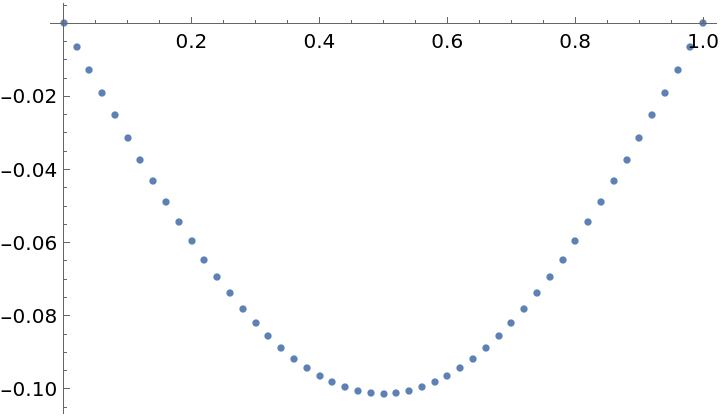 |
Plot the error:
| In[42]:= |
| Out[42]= | 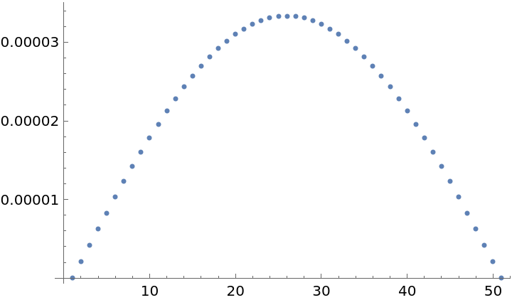 |
Solve the boundary value problem ![]() , using finite difference approximations on a non-uniform grid:
, using finite difference approximations on a non-uniform grid:
| In[43]:= | ![n = 50;
xgrid = With[{s = 2, xj = Range[0, n - 1]}, 0.5*(1 + (Tanh[s*((xj/Max[xj]) - 0.5)]/Tanh[s/2]))] ;
dx = Differences[xgrid]](https://www.wolframcloud.com/obj/resourcesystem/images/5e7/5e781cd2-a1b8-49a6-b730-92d3884266fb/72e1594939112881.png) |
| Out[45]= |  |
Generate the finite difference matrix for the second derivative:
| In[46]:= | ![fdres = ResourceFunction["FiniteDifferenceStencil"][
f''[x], {f[x - a], f[x], f[x + b]}, f, x];
coeffs = fdres["Coefficients"];
d2X = SparseArray[Join @@ Table[Block[{a, b},
{a, b} = dx[[i - 1 ;; i]];
Thread[{{i, i - 1}, {i, i}, {i, i + 1}} -> coeffs]
], {i, 2, n - 1}], {n, n}]](https://www.wolframcloud.com/obj/resourcesystem/images/5e7/5e781cd2-a1b8-49a6-b730-92d3884266fb/2ac0b91fa9aea957.png) |
| Out[48]= |
Modify the first and last row of the matrix to account for the boundary conditions:
| In[49]:= |
| Out[49]= |
Solve the discretized system:
| In[50]:= | ![rhs = Sin[Pi*xgrid];
rhs[[{1, -1}]] = 0.;
res = LinearSolve[d2X, rhs]](https://www.wolframcloud.com/obj/resourcesystem/images/5e7/5e781cd2-a1b8-49a6-b730-92d3884266fb/0f6da8e35cb9de64.png) |
| Out[52]= |  |
Plot the result:
| In[53]:= |
| Out[53]= | 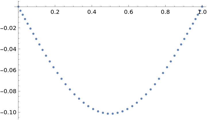 |
Plot the error:
| In[54]:= |
| Out[54]= | 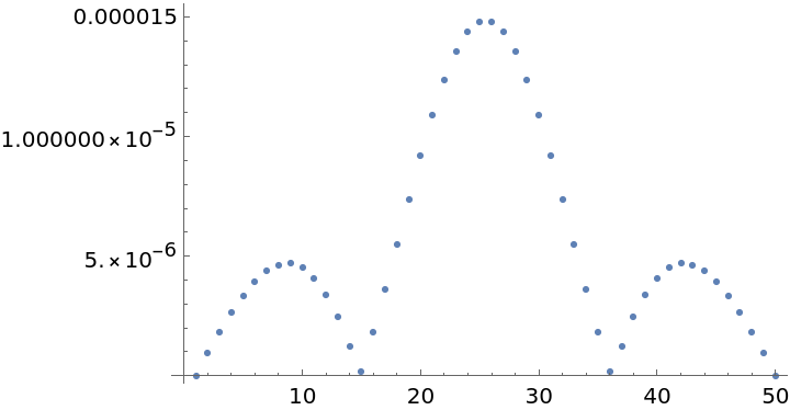 |
Solve the boundary value problem ![]() , using higher order compact finite difference approximations on a non-uniform grid:
, using higher order compact finite difference approximations on a non-uniform grid:
| In[55]:= | ![n = 50;
xgrid = With[{s = 2, xj = Range[0, n - 1]}, 0.5*(1 + (Tanh[s*((xj/Max[xj]) - 0.5)]/Tanh[s/2]))] ;
dx = Differences[xgrid]](https://www.wolframcloud.com/obj/resourcesystem/images/5e7/5e781cd2-a1b8-49a6-b730-92d3884266fb/2c1ae8492c52109b.png) |
| Out[57]= |  |
The finite difference stencil will consist of the functions and the second derivatives spanning three points:
| In[58]:= |
| Out[59]= |
The discretized higher order system will take the form ![]() Generate the matrix A:
Generate the matrix A:
| In[60]:= | ![acoeffs = coeffs[[1 ;; 3]];
A = SparseArray[Join @@ Table[Block[{a, b},
{a, b} = dx[[i - 1 ;; i]];
Thread[{{i, i - 1}, {i, i}, {i, i + 1}} -> acoeffs]
], {i, 2, n - 1}], {n, n}]](https://www.wolframcloud.com/obj/resourcesystem/images/5e7/5e781cd2-a1b8-49a6-b730-92d3884266fb/3cc91384c7c1617b.png) |
| Out[61]= |
Generate the matrix B:
| In[62]:= | ![bcoeffs = {-coeffs[[4]], 1, -coeffs[[5]]};
B = SparseArray[Join @@ Table[Block[{a, b},
{a, b} = dx[[i - 1 ;; i]];
Thread[{{i, i - 1}, {i, i}, {i, i + 1}} -> bcoeffs]
], {i, 2, n - 1}], {n, n}]](https://www.wolframcloud.com/obj/resourcesystem/images/5e7/5e781cd2-a1b8-49a6-b730-92d3884266fb/6411cf583a35d855.png) |
| Out[63]= |
Modify the first and last row of the matrices A, B to account for the boundary conditions:
| In[64]:= |
Solve the discretized system ![]() which is equal to
which is equal to ![]() :
:
| In[65]:= | ![rhs = Sin[Pi*xgrid];
rhs[[{1, -1}]] = 0.;
res = LinearSolve[A, B . rhs]](https://www.wolframcloud.com/obj/resourcesystem/images/5e7/5e781cd2-a1b8-49a6-b730-92d3884266fb/142f90cd7de876a7.png) |
| Out[67]= |  |
Plot the result:
| In[68]:= |
| Out[68]= |  |
The error is significantly better for the compact scheme:
| In[69]:= |
| Out[69]= | 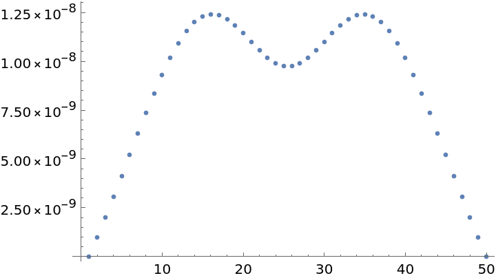 |
Use finite difference approximations to generate a variable step time integrator within NDSolve for solving ordinary differential equations. Use 4th and 5th order approximations of the function. The approximations are implicit because they use the first and second derivatives of the function at time t:
| In[70]:= |
| Out[70]= |
| In[71]:= |
| Out[71]= |  |
Set up the initialization of the method:
| In[72]:= | ![ImplicitFD45[___]["StepInput"] = {"F"["T", "X"], "H", "T", "X", "XP"};
ImplicitFD45[___]["StepOutput"] = {"H", "XI", "OBJ"};
ImplicitFD45[___]["DifferenceOrder"] = 4;
ImplicitFD45[___]["StepMode"] = Automatic;
ImplicitFD45 /: NDSolve`InitializeMethod[ImplicitFD45, stepmode_, sd_, rhs_, state_, opts___] := Module[{scalednorm, prec, rho, alp, coeffs1, coeffs2, f, t, h},
scalednorm = state["Norm"];
prec = state["WorkingPrecision"];
rho = N[8/10, prec];
alp = N[999/1000, prec];
coeffs1[h_] = Insert[ResourceFunction["FiniteDifferenceStencil"][
f[t], {f[t - h], f'[t - h], f'[t], f''[t]}, f, t][
"Coefficients"], 0, 3];
coeffs2[h_] = ResourceFunction["FiniteDifferenceStencil"][
f[t], {f[t - h], f'[t - h], f''[t - h], f'[t], f''[t]}, f, t][
"Coefficients"];
ImplicitFD45[scalednorm, {alp, rho, coeffs1, coeffs2}, {0, 0}]
];](https://www.wolframcloud.com/obj/resourcesystem/images/5e7/5e781cd2-a1b8-49a6-b730-92d3884266fb/2aecd57971bce715.png) |
Generate the step function. The next time step is computed based on the error between the fourth and fifth order approximation and a PI controller. Picard iterations are used to solve the implicit system:
| In[73]:= | ![ImplicitFD45[
scalednorm_, {alp_, rho_, coeffs1_, coeffs2_}, {errprv_, hprv_}][
"Step"[rhs_, h_, t0_, x0_, xp0_]] := Catch[Module[{ jt, jx, xpp0, x1, x2, xprv, xp1, xpp1, coeffs, t1, err, h2, hnext, dx},
{jt, jx} = rhs["JacobianMatrix"[t0, x0, "InputIndex" -> #]] & /@ {"T", "X"};
xpp0 = jt + jx . xp0; x1 = xprv = x0 + h*xp0 + (h^2)*xpp0;
t1 = t0 + h;
coeffs = coeffs1[h];
{x1, x2} = Reap[Do[
Do[
xp1 = rhs[t1, x1];
{jt, jx} = rhs["JacobianMatrix"[t1, x1, "InputIndex" -> #]] & /@ {"T", "X"};
x1 = coeffs . {x0, xp0, xpp0, xp1, jt + jx . xp1};
err = scalednorm[x1 - xprv, x1];
If[err <= 1, Break[]];
xprv = x1;
, {iter, 10}];
If[err >= 1, Break[]];
Sow[x1]; coeffs = coeffs2[h];
, {2}]][[2, 1]];
h2 = h;
If[err <= 1, err = scalednorm[x2 - x1, x2] + 10^-15];
If[err > 1, {hnext, dx, err, h2} = {h/Min[err, 2], $Failed, errprv, hprv};
,
hnext = If[hprv == 0, Max[h/2, Min[11*h/10, rho*(1/err)^(1/5)]],
Max[h/2, Min[11*h/10, rho*((h^2)/hprv)*((alp*errprv)/(err^2))^(1/5)]]];
dx = x2 - x0;
];
{hnext, dx, ImplicitFD45[
scalednorm, {alp, rho, coeffs1, coeffs2}, {err, h2}]}
]]](https://www.wolframcloud.com/obj/resourcesystem/images/5e7/5e781cd2-a1b8-49a6-b730-92d3884266fb/37c53d28697cbdf2.png) |
Solve the Lorenz system using the new variable step solver:
| In[74]:= | ![{res, dr} = Reap[NDSolve[{x'[t] == -3 (x[t] - y[t]), y'[t] == -x[t] z[t] + 28 x[t], z'[t] == x[t] y[t] - z[t], x[0] == 0, y[0] == 1, z[0] == 0}, {x, y, z}, {t, 0, 20}, Method -> ImplicitFD45, StepMonitor :> Sow[t]]]; res](https://www.wolframcloud.com/obj/resourcesystem/images/5e7/5e781cd2-a1b8-49a6-b730-92d3884266fb/010df4dc72796feb.png) |
| Out[74]= | 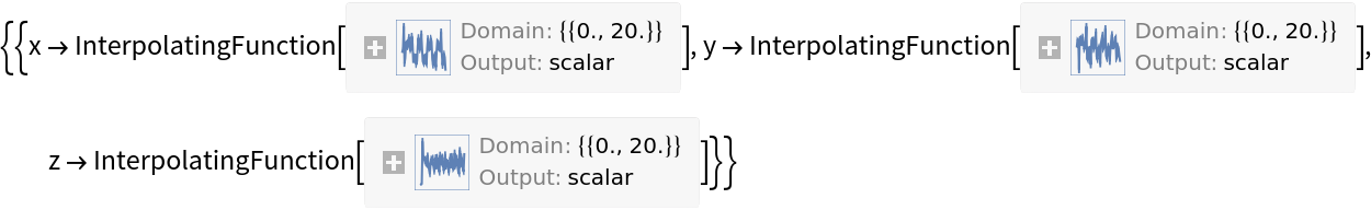 |
Plot the result:
| In[75]:= |
| Out[75]= | 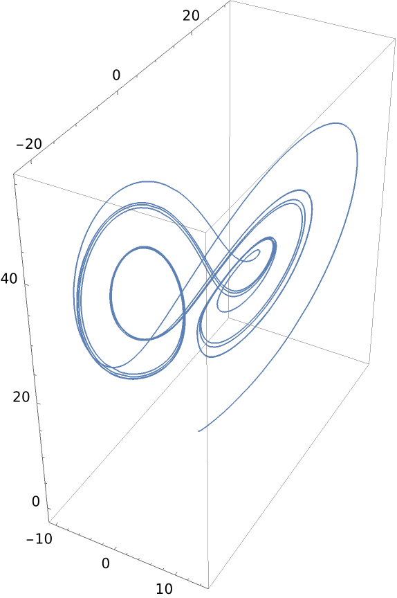 |
Plot the time-steps taken:
| In[76]:= |
| Out[76]= | 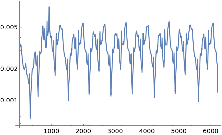 |
Use the variable step integrator to solve an ODE whose exact solution is known:
| In[77]:= | ![Remove[exact, rhs];
exact[t_] := Sin[2 Pi Exp[-Cos[t]^3] + t];
rhs[y_, t_] = Cos[y] + (D[exact[t], t] - Cos[exact[t]])](https://www.wolframcloud.com/obj/resourcesystem/images/5e7/5e781cd2-a1b8-49a6-b730-92d3884266fb/48f671c9ce690a49.png) |
| Out[78]= |
Solve the ODE:
| In[79]:= | ![{sol, rr} = Reap[NDSolveValue[{y'[t] == rhs[y[t], t], y[0] == exact[0]}, y, {t, 0, 10}, Method -> ImplicitFD45, StepMonitor :> Sow[t]]];
sol](https://www.wolframcloud.com/obj/resourcesystem/images/5e7/5e781cd2-a1b8-49a6-b730-92d3884266fb/47690ad136cf1704.png) |
| Out[80]= |
The error between the exact and approximated solution should be within the default tolerance of 10-8:
| In[81]:= |
| Out[81]= | 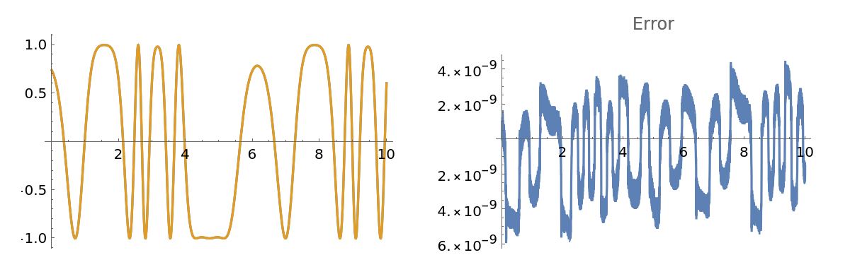 |
Plot the time steps used:
| In[82]:= |
| Out[82]= | 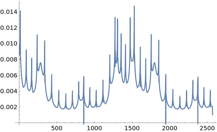 |
A finite difference stencil may not be obtained if sufficient stencils are not provided:
| In[83]:= |
| Out[84]= |
For certain stencil positions, a finite difference formula cannot be obtained:
| In[85]:= |
| Out[85]= |
This work is licensed under a Creative Commons Attribution 4.0 International License