Wolfram Function Repository
Instant-use add-on functions for the Wolfram Language
Function Repository Resource:
Get a numerically sorted list of abscissa-weight pairs for Fejér quadrature
ResourceFunction["FejerQuadratureWeights"][m,n,{a,b}] gives a list of the n pairs {xi,wi} of the n-point Fejér formula for quadrature of type m on the interval a to b, where wi is the weight of the abscissa xi. | |
ResourceFunction["FejerQuadratureWeights"][m,n,{a,b},prec] uses the working precision prec. |
The abscissas and weights for a 10-point type-1 Fejér quadrature on a given interval:
| In[1]:= |
|
| Out[1]= |
|
The abscissas and weights for a 10-point type-2 Fejér quadrature on a given interval:
| In[2]:= |
|
| Out[2]= |
|
Use the specified precision:
| In[3]:= |
|
| Out[3]= |
|
Use "I" or "II" to specify the type of Fejér quadrature:
| In[4]:= |
|
| Out[4]= |
|
| In[5]:= |
|
| Out[5]= |
|
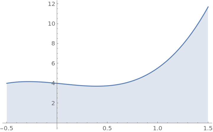
Use Fejér quadrature to approximate the area under a curve. First define a function:
| In[6]:= |
|
| Out[6]= |
|
Plot the curve over a given interval:
| In[7]:= |
|
| Out[7]= |
|
Approximate the area under the curve using n-point type-1 Fejér quadrature:
| In[8]:= |
![fejerArea1[n_] := Module[{a, w}, {a, w} = Transpose@
ResourceFunction["FejerQuadratureWeights"][1, n, {-0.5, 1.5}]; w.(f /@ a)]](https://www.wolframcloud.com/obj/resourcesystem/images/efa/efa0c19d-dbf5-441d-a0aa-c743436ac8e4/0cc687a36391f943.png)
|
| In[9]:= |
|
| Out[9]= |
|
Compare to the output of NIntegrate:
| In[10]:= |
|
| Out[10]= |
|
| In[11]:= |
|
| Out[11]= |
|
Approximate the area under the curve using n-point type-2 Fejér quadrature:
| In[12]:= |
![fejerArea2[n_] := Module[{a, w}, {a, w} = Transpose@
ResourceFunction["FejerQuadratureWeights"][2, n, {-0.5, 1.5}]; w.(f /@ a)]](https://www.wolframcloud.com/obj/resourcesystem/images/efa/efa0c19d-dbf5-441d-a0aa-c743436ac8e4/3e055f684d2cfab5.png)
|
| In[13]:= |
|
| Out[13]= |
|
Compare to the output of NIntegrate:
| In[14]:= |
|
| Out[14]= |
|
| In[15]:= |
|
| Out[15]= |
|
The abscissas of type-1 n-point Fejér quadrature are the roots of the Chebyshev polynomial Tn(x):
| In[16]:= |
|
| Out[16]= |
|
| In[17]:= |
|
| Out[17]= |
|
The abscissas of type-2 n-point Fejér quadrature are the extrema of the Chebyshev polynomial Tn+1(x):
| In[18]:= |
|
| Out[18]= |
|
| In[19]:= |
|
| Out[19]= |
|
This work is licensed under a Creative Commons Attribution 4.0 International License