Function Repository Resource:

DihedralODE

Source Notebook

Find the ordinary differential equation constraining periods of certain symmetrical curves

Contributed by: Bradley Klee

ResourceFunction["DihedralODE"][H,{λ,ϕ,α}]

returns the ODE constraining integral periods T(α), given a Hamiltonian H such that α=H(λ,cos(k ϕ)).

ResourceFunction["DihedralODE"][H,{λ,ϕ,α},rules]

first applies coordinate rewrite rules to H.

ResourceFunction["DihedralODE"][H,"Certificate"]

assumes default coordinate handling and returns a checked and checkable Association containing proof data.

Details

The acronym ODE stands for "ordinary differential equation."

Specification of variables {λ,ϕ,α} is optional if the Hamiltonian is written in terms of the formal action-angle variables

Input Hamiltonian H should be polynomial in

and linear in

, something like

Input Hamiltonian H can also be specified in Cartesian (p,q) or spherical (X,Y,Z) coordinates.

Spherical curves are drawn on the surface of a unit sphere, X²+Y²+Z²=1.

The default rewrite rules change from either system to action-angle coordinates:

Cartesian

Spherical

Note: Both the plane and the sphere are symplectic manifolds with canonical action-angle coordinates.

Time t is defined in terms of the tangents D_t{λ,ϕ}={-∂_ϕH,∂_λH}.

The invariant time differential may then be written most directly as dt=dϕ/(∂_λH).

Subsequent α-derivatives of the integrand dt are written as (∂_α)ⁿdt=(∂_λH)dt(∂_α)ⁿ1/(∂_λH).

Here we operate ∂_α through λ via the chain rule with ∂_αλ=1/(∂_λH). For example: ∂_αf(α, λ(α))=f^(1,0)(α,λ(α))+f^(0,1)(α, λ(α))/(∂_λH).

The primary task of ResourceFunction["DihedralODE"] is to compute a set of coefficients c_n(α) and a certificate Ξ(q,p) such that

. When this condition is satisfied, the exact differential can be integrated to zero around a contour, which implies

The form of the minimal output is an ordinary differential equation constraining period functions T(α).

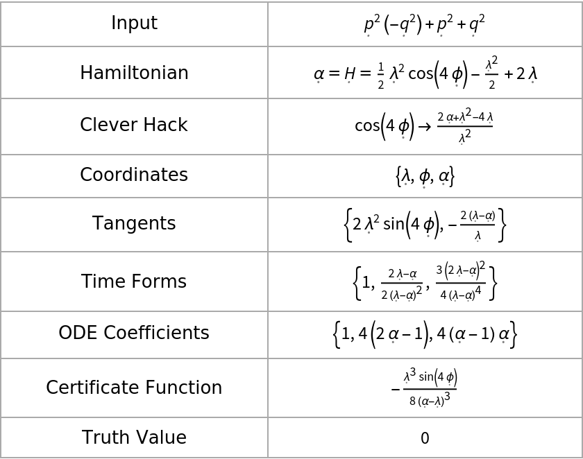
The proof data described above can be put into an Association:

PastedInput

Hamiltonian

α=H

Coordinates

{λ,ϕ,α}

Tangents

{-∂_ϕH,∂_λH}

Time Forms

(∂_α)ⁿdt,n=0, 1, …

ODE Coefficients

c_n,n=0, 1, …

Certificate Function

Truth Value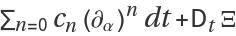

The last item with the key "Truth Value" should auto-evaluate to 0 for valid data.

For more details refer to "An Update on the Computational Theory of Hamiltonian Period Functions," especially Chapter 3.

By applying a clever hack, ∂_λH can be written as a ratio of λ-polynomials. If it succeeds, the algorithm should proceed rapidly to a solution, whereas if it fails the algorithm stops.

Caveat emptor: This function is effective for a few interesting results but comes with no warranty otherwise!

Examples

Basic Examples (3)

Find the period ODE coefficients of a family of elliptic curves in Edwards's normal form:

In[1]:=

$TraditionalForm[ ResourceFunction[ "DihedralODE"][\[FormalP]^2 + \[FormalQ]^2 - \[FormalP]^2 \[FormalQ]^2]]$

Out[1]=

Solve the ODE to find the real-valued hypergeometric period function:

In[2]:=

$With[{hyper2F1pars = First[ Solve[# == 0 & /@ Flatten[CoefficientList[ ResourceFunction[ "DihedralODE"][\[FormalP]^2 + \[FormalQ]^2 - \[FormalP]^2 \[FormalQ]^2, True]["ODE Coefficients"] - {-a b, c - (a + b + 1) \[FormalAlpha], \[FormalAlpha] (1 - \[FormalAlpha])} k, \[FormalAlpha]]]]]}, TraditionalForm[\[FormalCapitalT][ \[FormalAlpha]] == Pi Hypergeometric2F1[a, b, c, \[FormalAlpha]] /. hyper2F1pars]]$

Out[2]=

Display the proof data in a table:

In[3]:=

$Grid[Transpose[{Text /@ Keys[#], TraditionalForm /@ Values[#]}], Frame -> All, FrameStyle -> Lighter@Gray, Spacings -> {5, 1} ] &@ResourceFunction[ "DihedralODE"][\[FormalP]^2 + \[FormalQ]^2 - \[FormalP]^2 \[FormalQ]^2, True]$

Out[3]=

Scope (1)

Despite imperfections, this flexible technique is still quite formidable:

In[4]:=

$With[{dihedralExamples = {\[FormalP]^2 + \[FormalQ]^2 - \[FormalP]^2 \[FormalQ]^2, ( 1 + Rational[-1, 4] \[FormalQ]^2) (\[FormalP]^2 + \[FormalQ]^2), \[FormalP]^2 + \[FormalQ]^2 + ( Rational[2, 3] 3^Rational[-1, 2]) (( 3 \[FormalP]^2) \[FormalQ] - \[FormalQ]^3), \[FormalP]^2 + \[FormalQ]^2 + ( Rational[ 4, 27] \[FormalP]^2) (\[FormalP]^2 - 3 \[FormalQ]^2)^2 + Rational[-4, 27] (\[FormalP]^2 + \[FormalQ]^2)^3, \[FormalP]^2 + \[FormalQ]^2 + ( 2 \[FormalP]^2) \[FormalQ]^2 + Rational[-1, 4] (\[FormalP]^2 + \[FormalQ]^2)^2, \[FormalP]^2 + \[FormalQ]^2 + Rational[-1, 4] (\[FormalP]^2 + \[FormalQ]^2)^2 + (\[FormalP]^2 \[FormalQ]^2) \[Epsilon], \[FormalP]^2 + \[FormalQ]^2 + Rational[-1, 4] (\[FormalP]^2 + \[FormalQ]^2)^2 + (( Rational[ 1, 4] \[FormalP]^2) (\[FormalP]^2 + \[FormalQ]^2)) \[Epsilon], \[FormalCapitalX]^2 a + \[FormalCapitalY]^2 b + \[FormalCapitalZ]^2 c, 2^Rational[-1, 2] (\[FormalCapitalX]^3 - ( 3 \[FormalCapitalX]) \[FormalCapitalY]^2) + \[FormalCapitalZ]^3 + Rational[-3, 2] (\[FormalCapitalX]^2 \[FormalCapitalZ] + \[FormalCapitalY]^2 \[FormalCapitalZ]), (4 \[FormalCapitalX]^2) \[FormalCapitalY]^2 + ( 4 \[FormalCapitalX]^2) \[FormalCapitalZ]^2 + ( 4 \[FormalCapitalY]^2) \[FormalCapitalZ]^2, (((-2) \[FormalCapitalX]) (\[FormalCapitalX]^4 - ( 10 \[FormalCapitalX]^2) \[FormalCapitalY]^2 + 5 \[FormalCapitalY]^4)) \[FormalCapitalZ] + ( 5 (\[FormalCapitalX]^2 + \[FormalCapitalY]^2)^2) \[FormalCapitalZ]^2 - ( 5 (\[FormalCapitalX]^2 + \[FormalCapitalY]^2)) \[FormalCapitalZ]^4 + \[FormalCapitalZ]^6, ((-\[FormalCapitalX]^2) \[FormalCapitalY]^2) \[FormalCapitalZ]^2 + Rational[-2, 27] (\[FormalCapitalX]^2 + \[FormalCapitalY]^2 + \[FormalCapitalZ]^2) + Rational[ 1, 3] (\[FormalCapitalX]^4 + \[FormalCapitalY]^4 + \[FormalCapitalZ]^4)}}, Column[Reverse@AbsoluteTiming[Grid[ With[{res = ResourceFunction["DihedralODE"][#, True]}, {res[ "Truth Value"], #}] & /@ dihedralExamples , Frame -> All, Spacings -> {4, 1}, FrameStyle -> LightGray]]]]$

Out[4]=

Properties and Relations (1)

Proof data is dynamically checkable in a short amount of time:

In[5]:=

$AnnihilationCondition[vars_, tans_, dtForms_, coefficients_, cert_, qVal_ ] := Factor[Plus[Dot[D[cert, #] & /@ vars[[1 ;; 2]], tans] /. {Cos[_] -> \[FormalCapitalQ], Sin[_] -> \[FormalCapitalP]} /. { \[FormalCapitalP] -> Sqrt[1 - \[FormalCapitalQ]^2]} /. {\[FormalCapitalQ] -> qVal}, dtForms . coefficients]]$

In[6]:=

$With[{proof = ResourceFunction["DihedralODE"][ \[FormalP]^2 + \[FormalQ]^2 - \[FormalP]^2 \[FormalQ]^2, True]}, AnnihilationCondition[ proof["Coordinates"], proof["Tangents"], proof["Time Forms"], proof["ODE Coefficients"], proof["Certificate Function"], proof["Clever Hack"][[2]] ]]$

Out[6]=

Possible Issues (2)

Hyperelliptic inputs with separable potentials should not be expected to parse:

In[7]:=

$ResourceFunction[ "DihedralODE"][\[FormalP]^2 + \[FormalQ]^2 - \[FormalQ]^3]$

Out[7]=

If output data becomes weighty, expect a time delay:

In[8]:=

$AbsoluteTiming[ ResourceFunction[ "DihedralODE"][\[FormalLambda] + \[FormalLambda]^2 Cos[ 4 \[FormalPhi]] + \[FormalLambda]^4 Cos[4 \[FormalPhi]]]]$

Out[8]=

Neat Examples (1)

Discover an apparent genus-degree relation:

In[9]:=

$(Length[ResourceFunction[ "DihedralODE"][\[FormalLambda] + \[FormalLambda]^(#/ 2) Cos[# \[FormalPhi]], True]["ODE Coefficients"]] - 1)/ 2 & /@ Range[3, 8]$