Wolfram Function Repository
Instant-use add-on functions for the Wolfram Language
Function Repository Resource:
Plot the decision boundaries of a classifier
ResourceFunction["DecisionBoundaryPlot"][data] plots the decision boundaries of a classifier trained on data. | |
ResourceFunction["DecisionBoundaryPlot"][data, classifier] plots the decision boundaries of a pre-trained ClassifierFunction classifier trained on data. |
| Method | Automatic | classification algorithm used to classify the data |
| "DataColors" | ColorData[97,"ColorList"] | color scheme representing data classes |
| PointSize | Large | size of points representing the data |
Generate labeled 2D data:
| In[1]:= |
| Out[1]= |
Plot their classification regions:
| In[2]:= |
| Out[2]= | 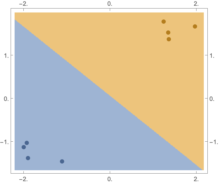 |
Generate labeled 2D data with three class labels:
| In[3]:= |
| Out[3]= |  |
Plot their classification boundaries:
| In[4]:= |
| Out[4]= | 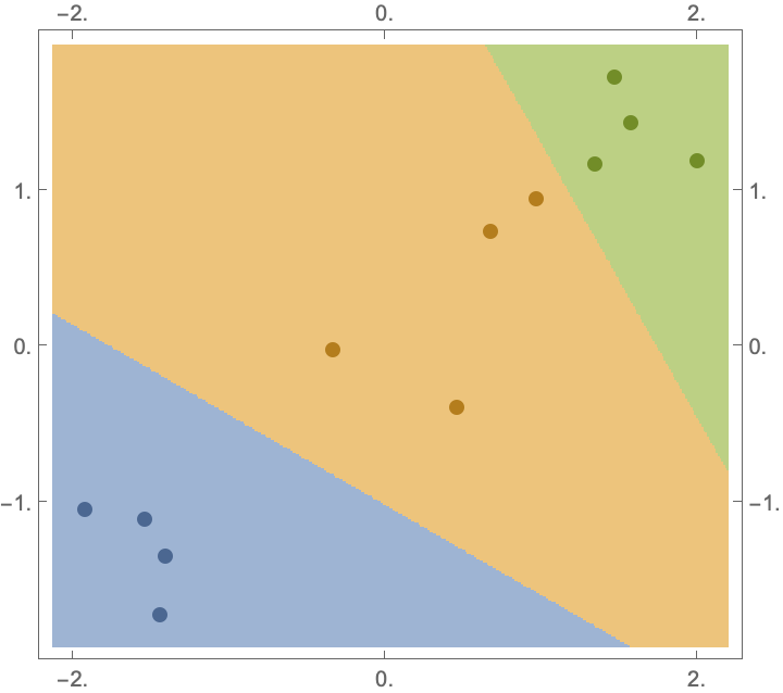 |
Plot the classification boundary of data as a List of rules:
| In[5]:= |
| Out[5]= | 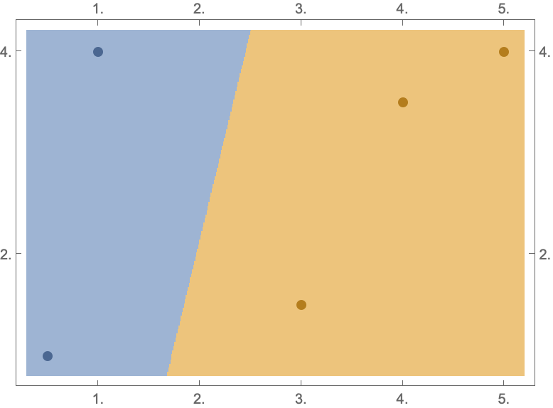 |
Plot the classification boundary of data as a Rule between points and classes:
| In[6]:= |
| Out[6]= | 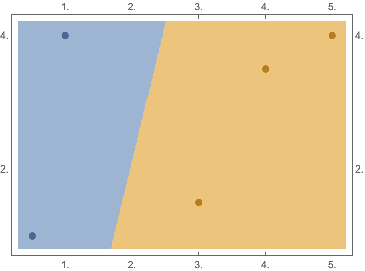 |
Generate clusters of 2D data:
| In[7]:= | ![cluster1 = RandomVariate[MultinormalDistribution[{0, 0}, IdentityMatrix[2]], 200];
cluster2 = MapThread[{#1 Cos[#2], #1 Sin[#2]} &, {RandomReal[{4, 5}, 200], RandomReal[{0, 2 Pi}, 200]}];
cluster3 = MapThread[{#1 Cos[#2], #1 Sin[#2]} &, {RandomReal[{6, 7}, 200], RandomReal[{0, 2 Pi}, 200]}];
data = <|1 -> cluster1, 2 -> cluster2, 3 -> cluster3|>;](https://www.wolframcloud.com/obj/resourcesystem/images/176/17642d9f-3153-49b8-91d4-c9b9057f07c1/1b674c62da792c7e.png) |
Classify the data:
| In[8]:= |
| Out[8]= |
Plot the decision regions:
| In[9]:= |
| Out[9]= | 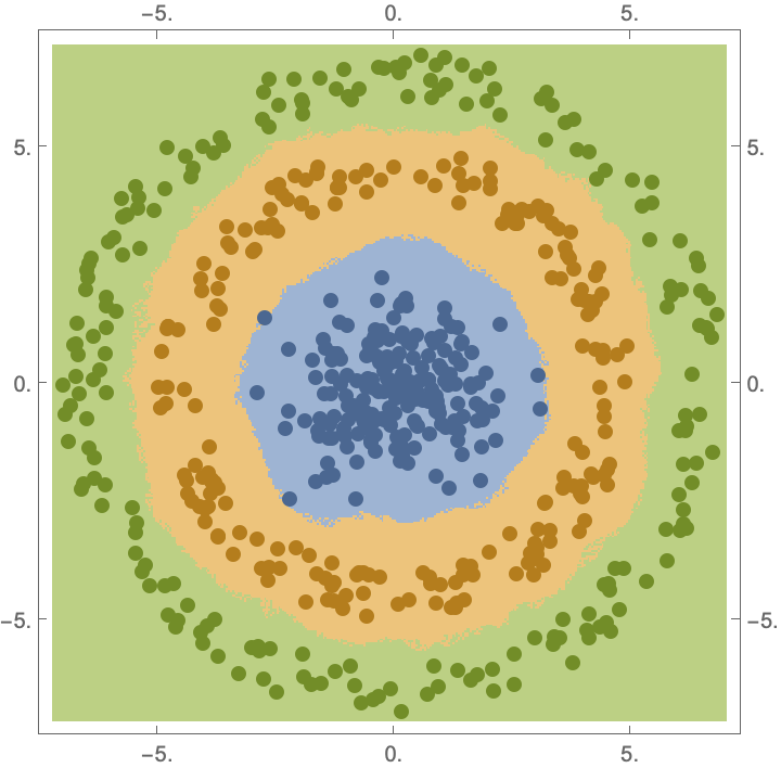 |
Generate data and use the Method option to specify the classification algorithm used to classify the data:
| In[10]:= |
| Out[10]= |  |
| In[11]:= |
| Out[11]= | 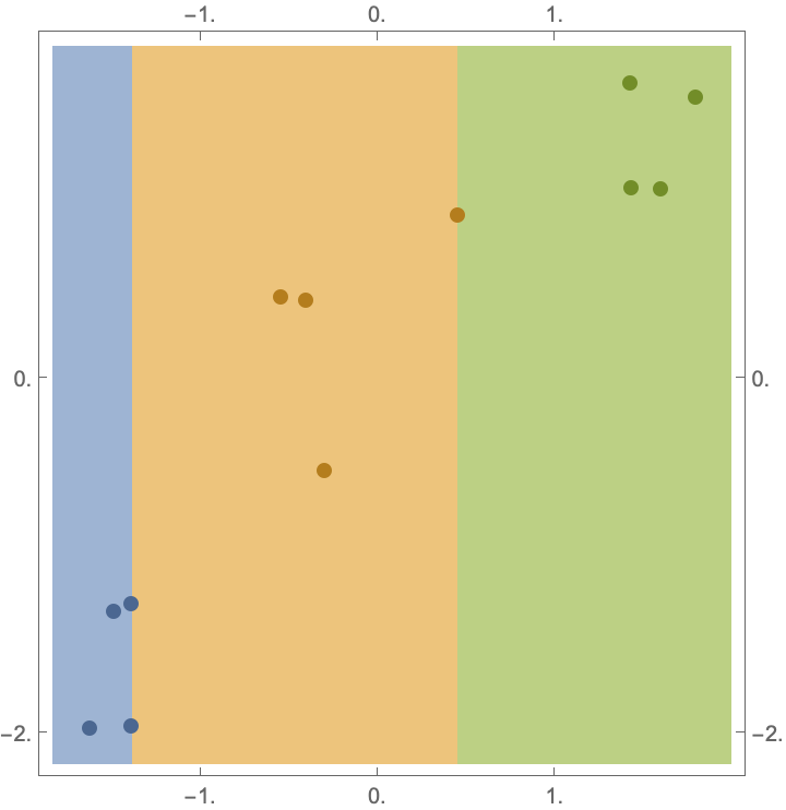 |
Compare it with a different classification method:
| In[12]:= |
| Out[12]= | 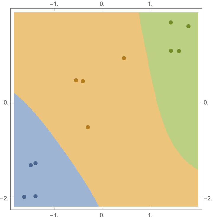 |
Change the color of each class using the "DataColors" option:
| In[13]:= |
| In[14]:= |
| Out[14]= | 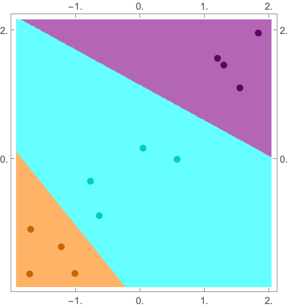 |
Change the size of data points with the PointSize option:
| In[15]:= |
| In[16]:= |
| Out[16]= | 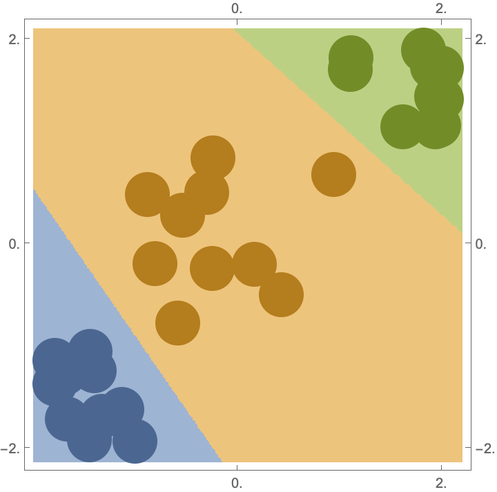 |
Generate data and compare different classification algorithms:
| In[17]:= | ![data = Flatten[Table[Module[{\[Mu], \[Sigma], pts},
\[Mu] = RandomReal[{-3, 3}, 2];
\[Sigma] = 0.2;
pts = RandomVariate[
MultinormalDistribution[\[Mu], \[Sigma] IdentityMatrix[2]], 10];
Rule @@@ Thread[pts -> ConstantArray[class, Length[pts]]]], {class, {"A",
"B", "C"}}], 1];](https://www.wolframcloud.com/obj/resourcesystem/images/176/17642d9f-3153-49b8-91d4-c9b9057f07c1/43f8e433c0a73009.png) |
| In[18]:= | ![With[{methods = {"LogisticRegression", "NeuralNetwork", "RandomForest",
"SupportVectorMachine"}}, GraphicsGrid[
Partition[
Table[ResourceFunction["DecisionBoundaryPlot"][data, Method -> method, PlotLabel -> method], {method, methods}], 2]]]](https://www.wolframcloud.com/obj/resourcesystem/images/176/17642d9f-3153-49b8-91d4-c9b9057f07c1/3d785146613316e3.png) |
| Out[18]= | 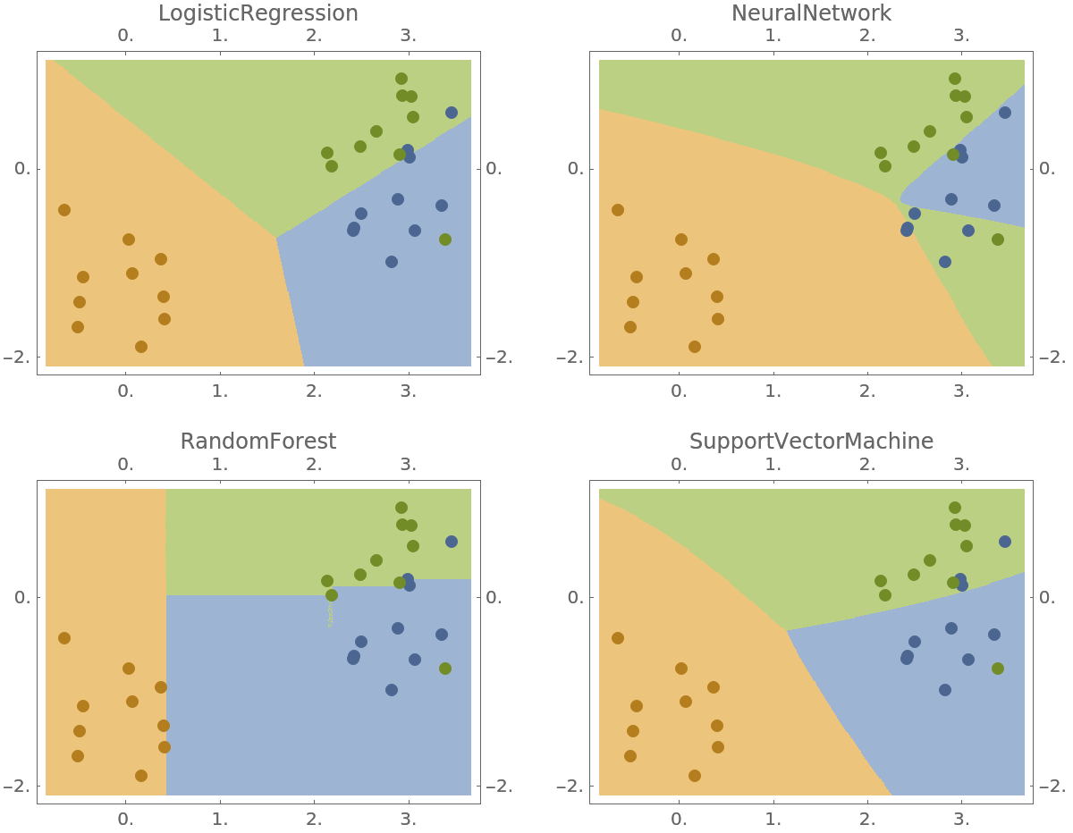 |
Each classification method accepts its own suboptions. Use the Method option to specify them and visualize how the classification regions change:
| In[19]:= | ![cluster1 = RandomVariate[MultinormalDistribution[{0, 0}, IdentityMatrix[2]], 200];
cluster2 = MapThread[{#1 Cos[#2], #1 Sin[#2]} &, {RandomReal[{4, 5}, 200], RandomReal[{0, 2 Pi}, 200]}];
data = <|1 -> cluster1, 2 -> cluster2|>;](https://www.wolframcloud.com/obj/resourcesystem/images/176/17642d9f-3153-49b8-91d4-c9b9057f07c1/04f07673aa28946c.png) |
| In[20]:= | ![With[{kernelTypes = {"Linear", "RadialBasisFunction"}}, GraphicsGrid[{Table[
ResourceFunction["DecisionBoundaryPlot"][data, Method -> {"SupportVectorMachine", "KernelType" -> kernelType}, PlotLabel -> "SVM, " <> kernelType <> " kernel"], {kernelType, kernelTypes}]}]]](https://www.wolframcloud.com/obj/resourcesystem/images/176/17642d9f-3153-49b8-91d4-c9b9057f07c1/26ad26bf436a7b7c.png) |
| Out[20]= | 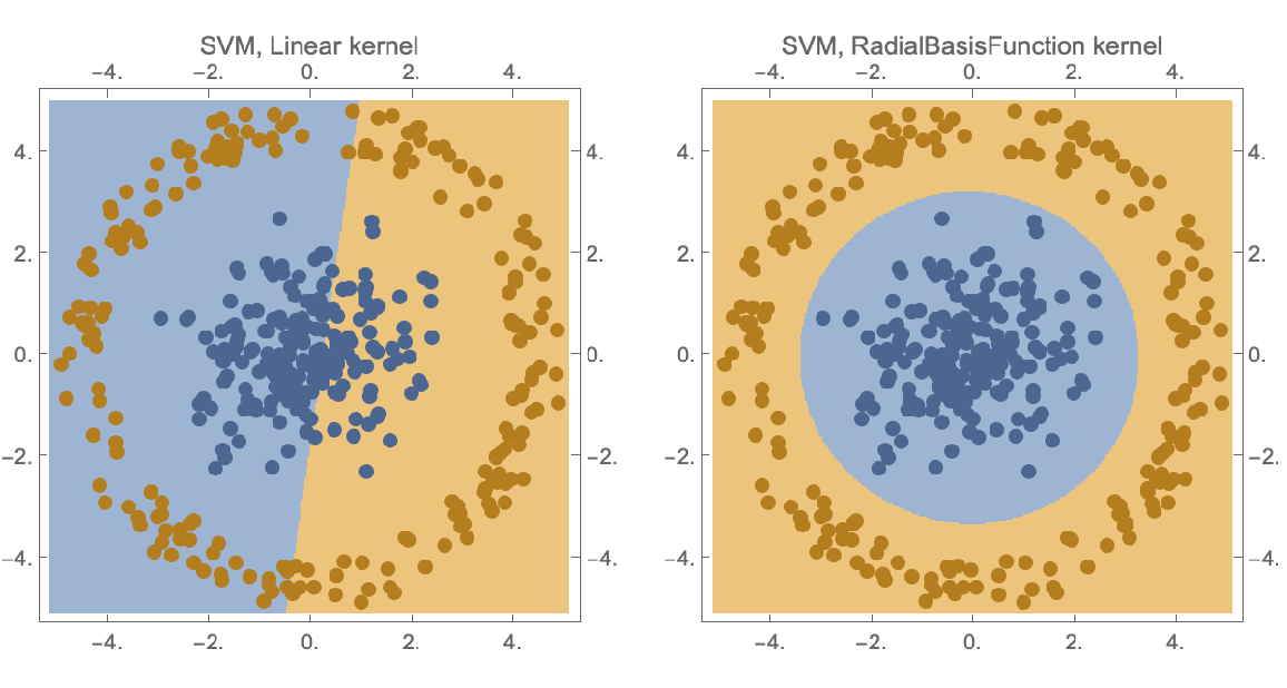 |
The training data must be two dimensional:
| In[21]:= |
| Out[21]= |
The training data must be labeled and formatted correctly:
| In[22]:= |
| Out[22]= |
Generate data for four different classes:
| In[23]:= | ![data = Flatten[Table[Module[{\[Mu], \[Sigma], pts},
\[Mu] = RandomReal[{-3, 3}, 2];
\[Sigma] = 0.2;
pts = RandomVariate[
MultinormalDistribution[\[Mu], \[Sigma] IdentityMatrix[2]], 15];
Rule @@@ Thread[pts -> ConstantArray[class, Length[pts]]]], {class, {"A",
"B", "C", "D"}}], 1];](https://www.wolframcloud.com/obj/resourcesystem/images/176/17642d9f-3153-49b8-91d4-c9b9057f07c1/30b16dac4e4366de.png) |
Specify different "GammaScalingParameter" values in the "SupportVectorMachine" classifier and notice how it overfits the data as this parameter increases:
| In[24]:= | ![With[{gammaValues = {0.1, 1, 10, 100}}, GraphicsGrid[
Partition[
Table[ResourceFunction["DecisionBoundaryPlot"][data, Method -> {"SupportVectorMachine", "KernelType" -> "RadialBasisFunction", "GammaScalingParameter" -> gamma}, PlotLabel -> \[Gamma] == gamma], {gamma, gammaValues}], 2]]]](https://www.wolframcloud.com/obj/resourcesystem/images/176/17642d9f-3153-49b8-91d4-c9b9057f07c1/13a235f1c9f19680.png) |
| Out[24]= | 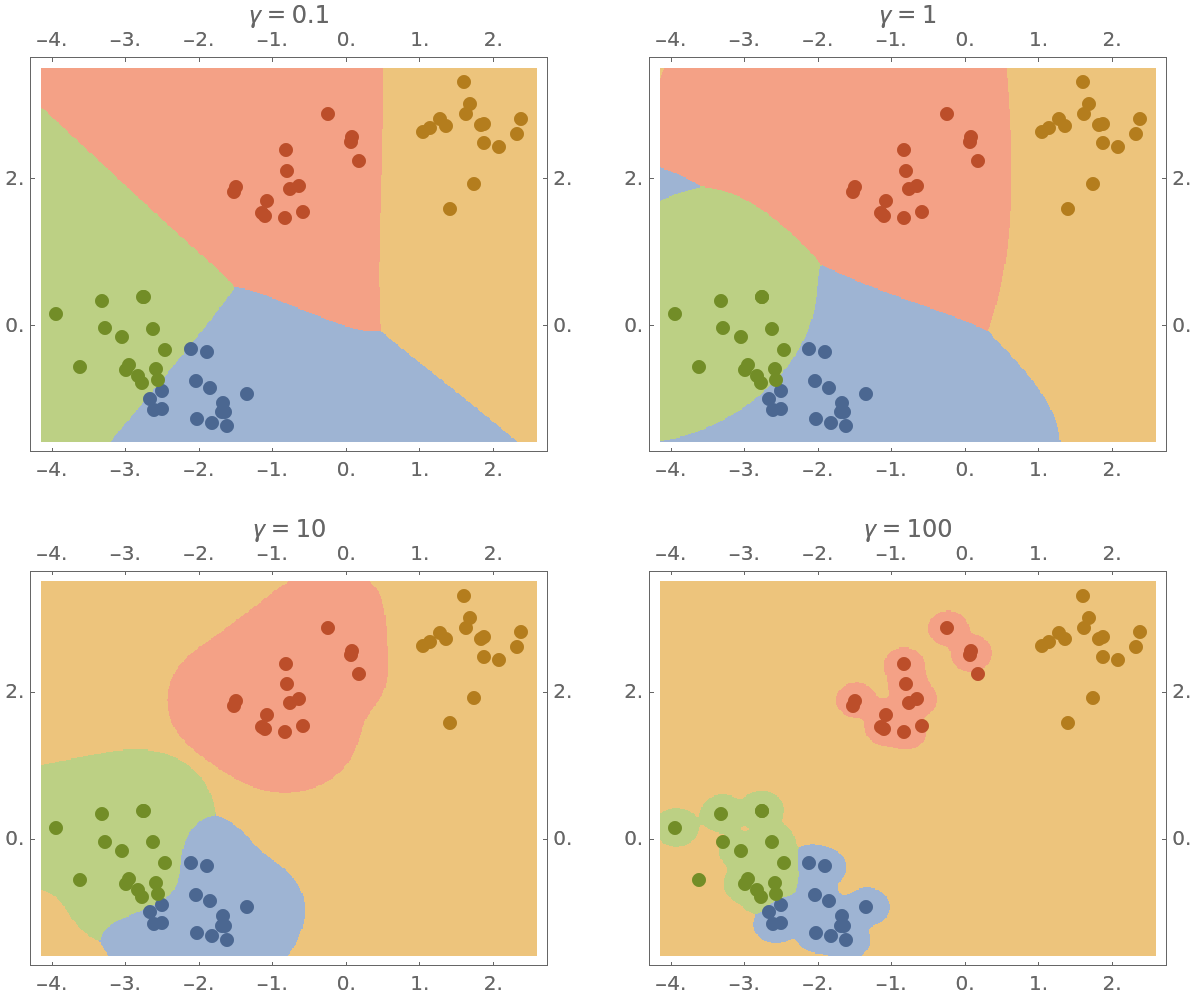 |
Wolfram Language 14.0 (January 2024) or above
This work is licensed under a Creative Commons Attribution 4.0 International License