Details and Options
ResourceFunction["CurveToBSplineFunction"] returns a
BSplineFunction object.
Before processing, successive duplicate points are removed from the input list of points {pt1,pt2,…}.
ResourceFunction["CurveToBSplineFunction"][{pt1,pt2,…},d] is equivalent to ResourceFunction["CurveToBSplineFunction"][{pt1,pt2,…},d,1].
The second argument
d determines the maximal degree of the underlying polynomial basis used by a
BSplineFunction object. Increasing this value leads to a smoother spline with fewer details.
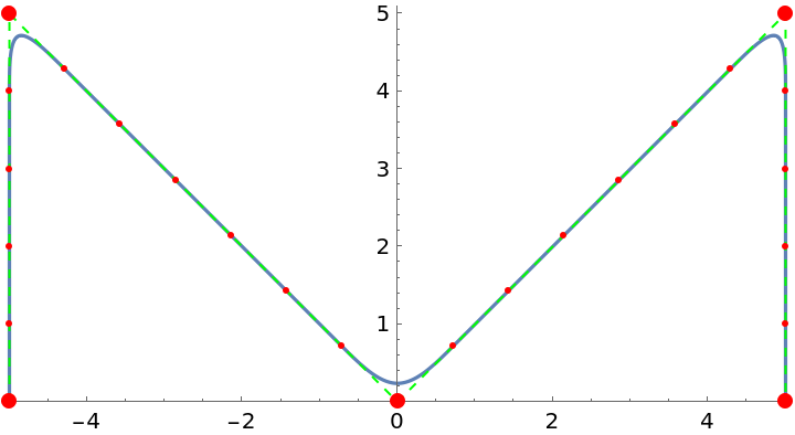
The third argument
scale is the scale factor used for filling the gaps between successive points of the curve when the option
"FillGaps"→True is set. With this setting,
equidistant control points will be introduced between the points
pti and
pti+1. By default, it is assumed that a scale of 1 means that no intermediate control points will be introduced when the Euclidean distance between successive points is less than 2. Increasing this value leads to a smoother spline with fewer details.
The following options can be given:
| "AssignWeights" | False | controls assigning weights to the control point of a generated spline |
| "CurveClosed" | False | whether to treat the input curve defined by points {pt1,pt2,…} as closed |
| "DuplicateNodes" | False | controls duplication of the input control points pti |
| "FillGaps" | True | whether to introduce intermediate control points |
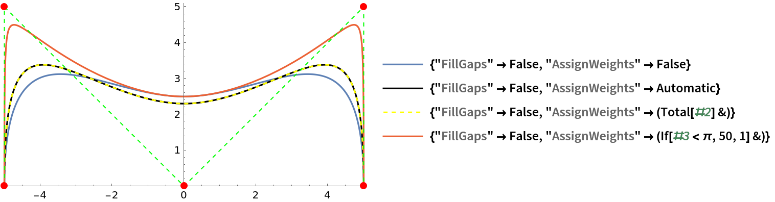
The option setting
"AssignWeights"→Automatic assigns to every control point of a generated spline the weight equal to the sum of its distances to the two adjacent points. With the setting
"AssignWeights"→f, where
f is a function, the weight of the point will be set to
f[pti, {l, r}, angle, scale]. This option helps to preserve the shape of the original curve by selectively increasing the weights of the control points.
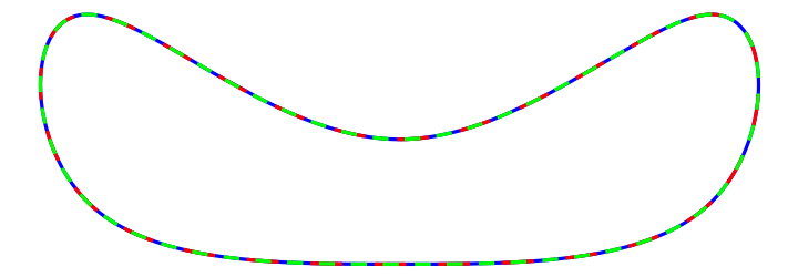
With the setting
"CurveClosed"→True, the input list of points
{pt1,pt2,…} is treated as cyclic.
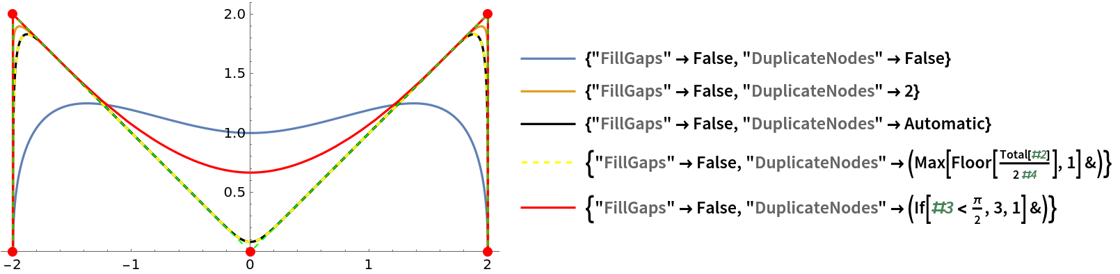
The option
"DuplicateNodes" gives flexible control over duplication of the input control points
pti inside of a produced
BSplineFunction. With the setting
"DuplicateNodes"→n, every point will be duplicated
n times. With the setting
"DuplicateNodes"→Automatic, every input point
pti will be duplicated
Max[Floor[(l+r)/(2 scale)],1] times, where
l and
r are Euclidean distances to the adjacent points from the left and the right, respectively. With
"DuplicateNodes"→f, where
f is a function, the point will be duplicated
f[pti, {l, r}, angle, scale] times, where
angle is the interior angle at the vertex point
pti (for the boundary points,
angle is set to
Infinity). This option allows preservation of the sharp corners of the original curve by duplicating the corresponding control points.
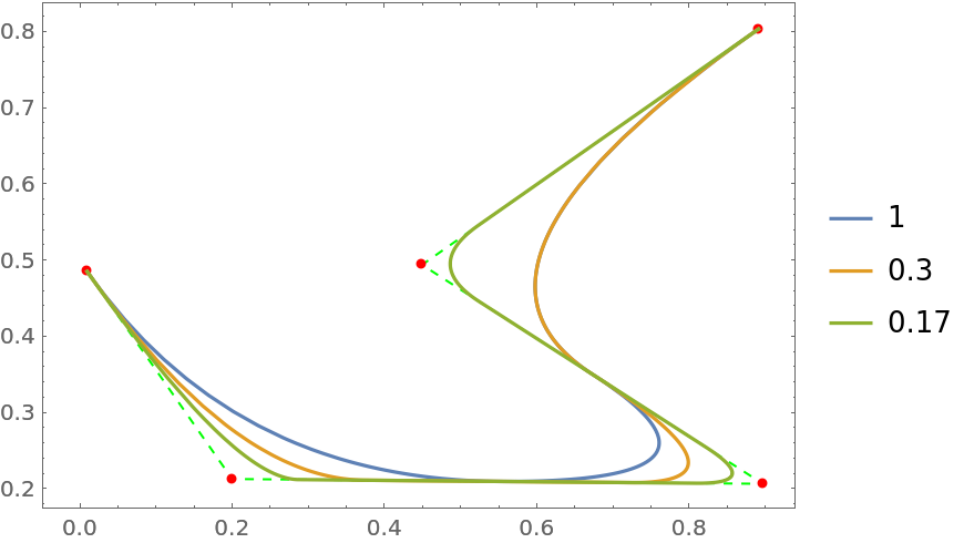
![SeedRandom[8];
curve = RandomReal[1, {5, 2}];
scales = {1, .3, .17};
functs = ResourceFunction["CurveToBSplineFunction"][curve, 2, #][\[FormalT]] & /@ scales;
ParametricPlot[functs, {\[FormalT], 0, 1}, Frame -> True, PlotLegends -> scales,
Prolog -> {Green, Dashed, Line[curve], Red, PointSize[Medium], Point[curve]}]](https://www.wolframcloud.com/obj/resourcesystem/images/98f/98f83926-bd08-423a-aa5f-7f67ec1af5b4/0165c1a90c9327a5.png)
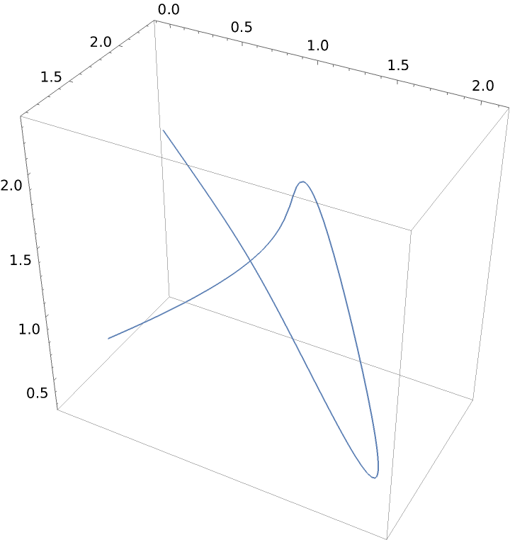
![SeedRandom[8];
g = ResourceFunction["CurveToBSplineFunction"][RandomReal[3, {6, 3}], 5]
ParametricPlot3D[g[u], {u, 0, 1}]](https://www.wolframcloud.com/obj/resourcesystem/images/98f/98f83926-bd08-423a-aa5f-7f67ec1af5b4/35373fc52a36587f.png)
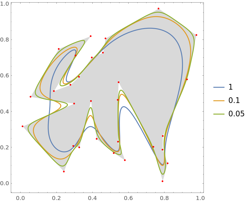
![SeedRandom[1];
nodes = RandomPolygon[{"Simple", 30}][[1]];
scales = {1, .1, .05};
functs = Table[
ResourceFunction["CurveToBSplineFunction"][nodes, 10, scale, "CurveClosed" -> True][\[FormalT]], {scale, scales}];
ParametricPlot[functs, {\[FormalT], 0, 1}, PlotLegends -> scales, Frame -> True, Epilog -> {Red, Point[nodes]}, Prolog -> {LightGray, Polygon[nodes]}]](https://www.wolframcloud.com/obj/resourcesystem/images/98f/98f83926-bd08-423a-aa5f-7f67ec1af5b4/0e81bf0514458bc9.png)
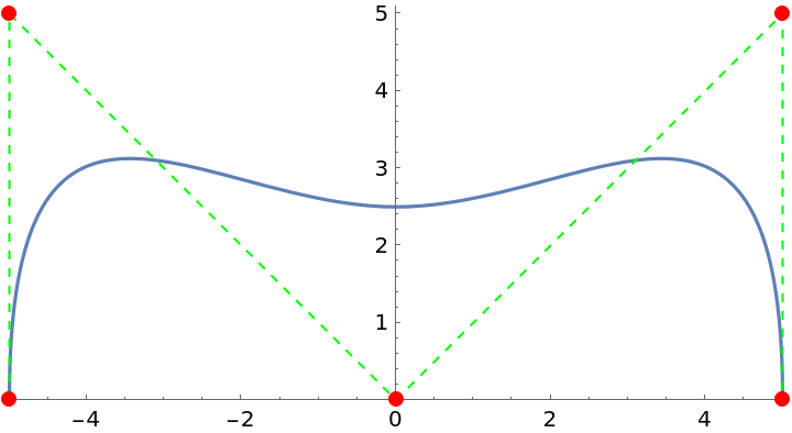
![nodes = 5 {{-1, 0}, {-1, 1}, {0, 0}, {1, 1}, {1, 0}};
opts = {"FillGaps" -> False, #} & /@
{"AssignWeights" -> False, "AssignWeights" -> Automatic, "AssignWeights" -> (Total[#2] &), "AssignWeights" -> (If[#3 < \[Pi], 50, 1] &)};
functs = ResourceFunction["CurveToBSplineFunction"][nodes, 3, #][\[FormalT]] & /@ opts;
ParametricPlot[functs, {\[FormalT], 0, 1}, Epilog -> {Green, Dashed, Line[nodes], Red, PointSize[Large], Point[nodes]}, PlotRange -> {{-5.1, 5.1}, {0, 5.1}}, PlotRangeClipping -> False, PlotLegends -> (Style[StandardForm@#, "Input", "Notebook", ShowSyntaxStyles -> True] & /@ opts), PlotStyle -> {Automatic, Black, {Yellow, Dashed}, Automatic}]](https://www.wolframcloud.com/obj/resourcesystem/images/98f/98f83926-bd08-423a-aa5f-7f67ec1af5b4/5ec36d442aab1964.png)
![nodes = {{-1, 0}, {-1, 1}, {0, 0}, {1, 1}, {1, 0}};
functs = ResourceFunction["CurveToBSplineFunction"][#, 3, "CurveClosed" -> True][\[FormalT]] & /@ {nodes, RotateLeft[nodes, 3], Reverse[nodes]};
ParametricPlot[functs, {\[FormalT], 0, 1}, Axes -> False, PlotStyle -> {Blue, {Red, Dashing[0.04]}, {Green, Dashing[0.02]}}]](https://www.wolframcloud.com/obj/resourcesystem/images/98f/98f83926-bd08-423a-aa5f-7f67ec1af5b4/02c53cda2ff1e7a1.png)
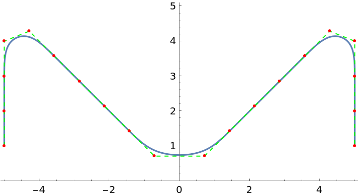
![nodes = 2 {{-1, 0}, {-1, 1}, {0, 0}, {1, 1}, {1, 0}};
opts = {"FillGaps" -> False, #} & /@
{"DuplicateNodes" -> False, "DuplicateNodes" -> 2, "DuplicateNodes" -> Automatic,
"DuplicateNodes" -> (Max[Floor[Total[#2]/(2 #4)], 1] &), "DuplicateNodes" -> (If[#3 < \[Pi]/2, 3, 1] &)};
functs = ResourceFunction["CurveToBSplineFunction"][nodes, 3, #][\[FormalT]] & /@ opts;
ParametricPlot[functs, {\[FormalT], 0, 1}, Epilog -> {Green, Dashed, Line[nodes], Red, PointSize[Large], Point[nodes]}, PlotRange -> {{-2.1, 2.1}, {0, 2.1}}, PlotRangeClipping -> False, PlotLegends -> (Style[StandardForm@#, "Input", "Notebook", ShowSyntaxStyles -> True] & /@ opts), PlotStyle -> {Automatic, Automatic, Black, {Yellow, Dashed}, Red}]](https://www.wolframcloud.com/obj/resourcesystem/images/98f/98f83926-bd08-423a-aa5f-7f67ec1af5b4/2923fe5bc8e67eb8.png)
![nodes = 5 {{-1, 0}, {-1, 1}, {0, 0}, {1, 1}, {1, 0}};
scale = 1;
f = ResourceFunction["CurveToBSplineFunction"][nodes, 3, scale];
ParametricPlot[f[t], {t, 0, 1}, Epilog -> {Green, Dashed, Line[nodes], Red, Point[f[[5, 1]]], PointSize[Large], Point[nodes]}, PlotRange -> {{-5.1, 5.1}, {0, 5.1}}, PlotRangeClipping -> False]](https://www.wolframcloud.com/obj/resourcesystem/images/98f/98f83926-bd08-423a-aa5f-7f67ec1af5b4/4a44b566ffdd9087.png)
![f = ResourceFunction["CurveToBSplineFunction"][nodes, 3, scale, "FillGaps" -> False];
ParametricPlot[f[t], {t, 0, 1}, Epilog -> {Green, Dashed, Line[nodes], Red, Point[f[[5, 1]]], PointSize[Large], Point[nodes]}, PlotRange -> {{-5.1, 5.1}, {0, 5.1}}, PlotRangeClipping -> False]](https://www.wolframcloud.com/obj/resourcesystem/images/98f/98f83926-bd08-423a-aa5f-7f67ec1af5b4/58ed38c653b4e7b2.png)
![f = ResourceFunction["CurveToBSplineFunction"][nodes, 3, 6];
ParametricPlot[f[t], {t, 0, 1}, Epilog -> {Green, Dashed, Line[nodes], Red, Point[f[[5, 1]]], PointSize[Large], Point[nodes]}, PlotRange -> {{-5.1, 5.1}, {0, 5.1}}, PlotRangeClipping -> False]](https://www.wolframcloud.com/obj/resourcesystem/images/98f/98f83926-bd08-423a-aa5f-7f67ec1af5b4/27439a8027d0caa5.png)

![f = ResourceFunction["CurveToBSplineFunction"][nodes, 3, scale, "DuplicateNodes" -> 0];
ParametricPlot[f[t], {t, 0, 1}, Epilog -> {Green, Dashed, Line[f[[5, 1]]], Red, Point[f[[5, 1]]]}, PlotRange -> {{-5.1, 5.1}, {0, 5.1}}, PlotRangeClipping -> False]](https://www.wolframcloud.com/obj/resourcesystem/images/98f/98f83926-bd08-423a-aa5f-7f67ec1af5b4/078857aaca37d3b4.png)
![img = Blur[
Rasterize[
Graphics[{Red, Rectangle[], Blue, Annulus[], Green, Triangle[{{-1, -1}, {0, -1}, {-1, 1}}]}, PlotRangePadding -> None], RasterSize -> 200], 5];
contours = Flatten[ComponentMeasurements[ClusteringComponents[img, 4], "Contours"][[2 ;;, 2]], 1];
Graphics[MapIndexed[{Thick, Opacity[.8], ColorData[97][#2[[1]]], #} &,
contours]]](https://www.wolframcloud.com/obj/resourcesystem/images/98f/98f83926-bd08-423a-aa5f-7f67ec1af5b4/5b9ed9dd80fd2344.png)
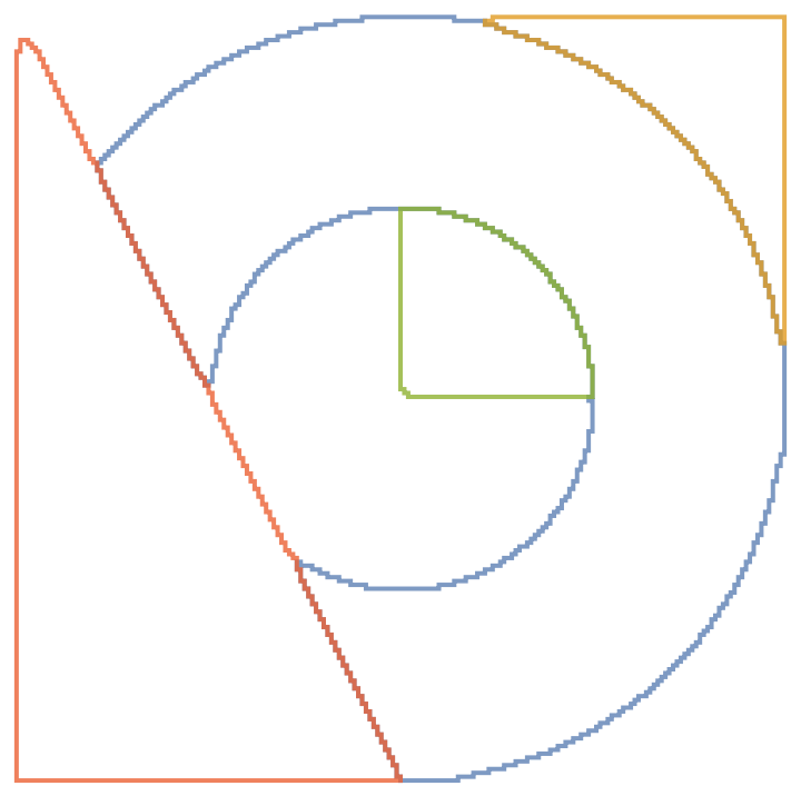
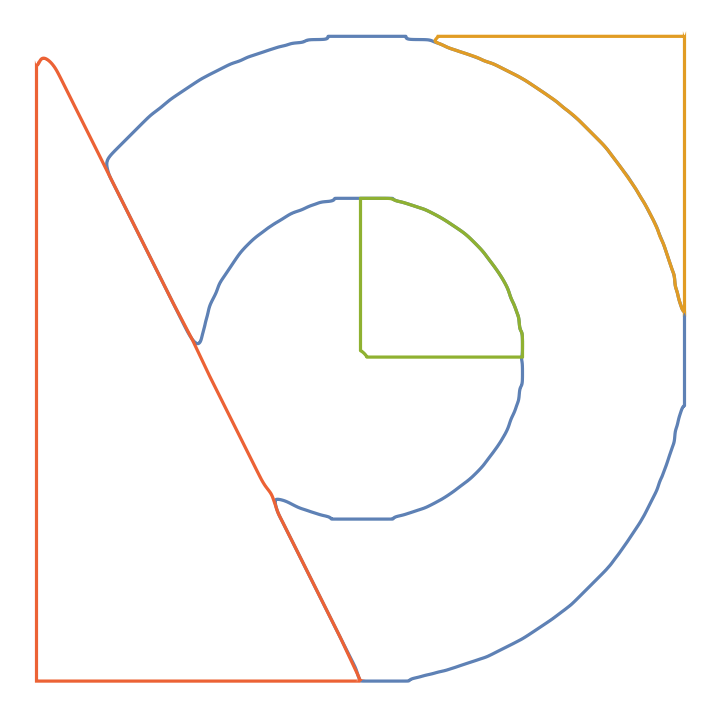
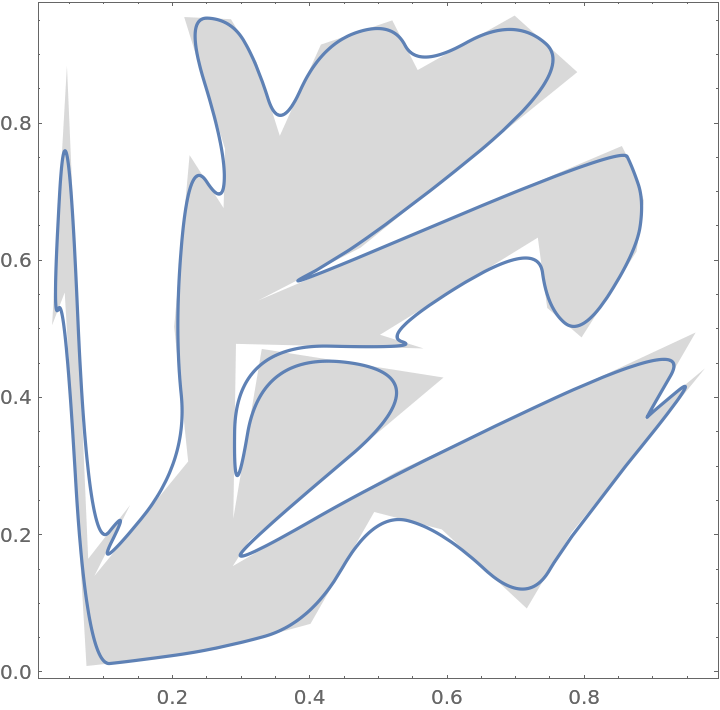
![functs = ResourceFunction["CurveToBSplineFunction"][#, 90, "CurveClosed" -> True,
"DuplicateNodes" -> Automatic][\[FormalT]] & @@@ contours;
ParametricPlot[functs, {\[FormalT], 0, 1}, Axes -> False]](https://www.wolframcloud.com/obj/resourcesystem/images/98f/98f83926-bd08-423a-aa5f-7f67ec1af5b4/74dc9e5ffb07296e.png)
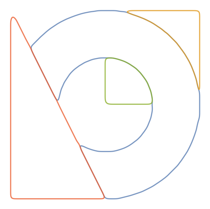
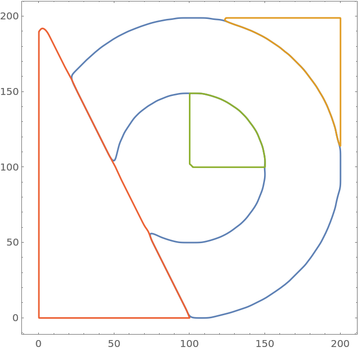
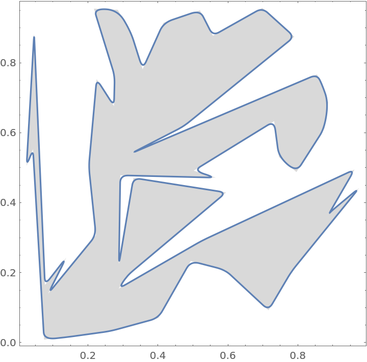
![functs = ResourceFunction["CurveToBSplineFunction"][#, 90, "CurveClosed" -> True,
"DuplicateNodes" -> (If[Max[#2] > 40 && #3 <= \[Pi]/2, 9, 1] &)][\[FormalT]] & @@@ contours;
ParametricPlot[functs, {\[FormalT], 0, 1}, Frame -> True]](https://www.wolframcloud.com/obj/resourcesystem/images/98f/98f83926-bd08-423a-aa5f-7f67ec1af5b4/1a3800e9eff21747.png)
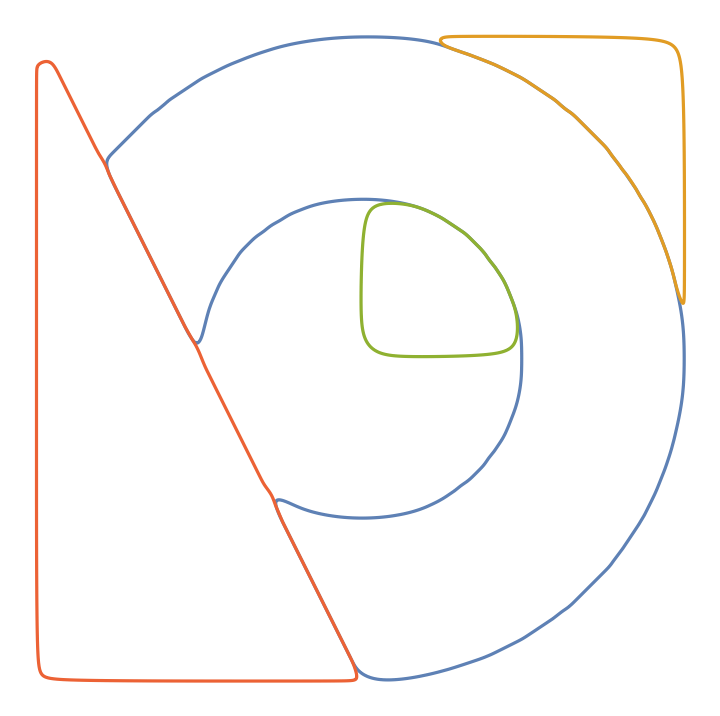
![functs = ResourceFunction["CurveToBSplineFunction"][#, 60,
"CurveClosed" -> True, "AssignWeights" -> Automatic][\[FormalT]] & @@@ contours;
ParametricPlot[functs, {\[FormalT], 0, 1}, Axes -> False]](https://www.wolframcloud.com/obj/resourcesystem/images/98f/98f83926-bd08-423a-aa5f-7f67ec1af5b4/4f6eeec4a2c4c240.png)

![functs = ResourceFunction["CurveToBSplineFunction"][#, 40, 10,
"CurveClosed" -> True, "AssignWeights" -> Automatic][\[FormalT]] & @@@ contours;
ParametricPlot[functs, {\[FormalT], 0, 1}, Axes -> False]](https://www.wolframcloud.com/obj/resourcesystem/images/98f/98f83926-bd08-423a-aa5f-7f67ec1af5b4/36817e6267897472.png)
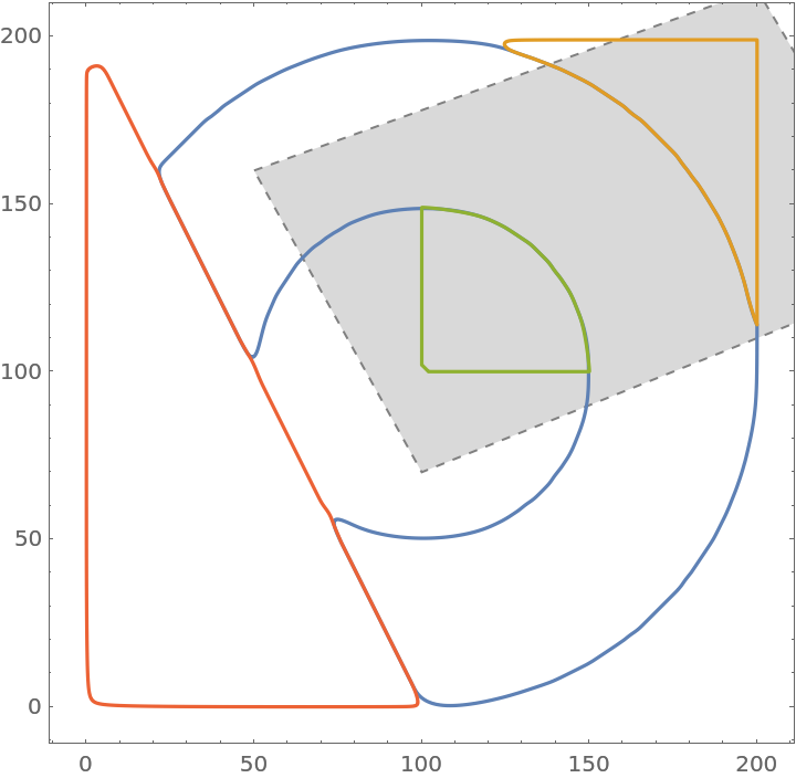
![region = Polygon[{{50, 160}, {200, 214}, {250, 130}, {100, 70}}];
mf = RegionMember[region];
functs = ResourceFunction["CurveToBSplineFunction"][#, 40, 10, "CurveClosed" -> True, "AssignWeights" -> Automatic,
"DuplicateNodes" -> (If[mf[#1] && Max[#2] > 20, 8, 1] &)][\[FormalT]] & @@@ contours;
ParametricPlot[functs, {\[FormalT], 0, 1}, Frame -> True, Prolog -> {FaceForm[LightGray], EdgeForm[{Gray, Dashed}], region}]](https://www.wolframcloud.com/obj/resourcesystem/images/98f/98f83926-bd08-423a-aa5f-7f67ec1af5b4/21266854aef8c583.png)
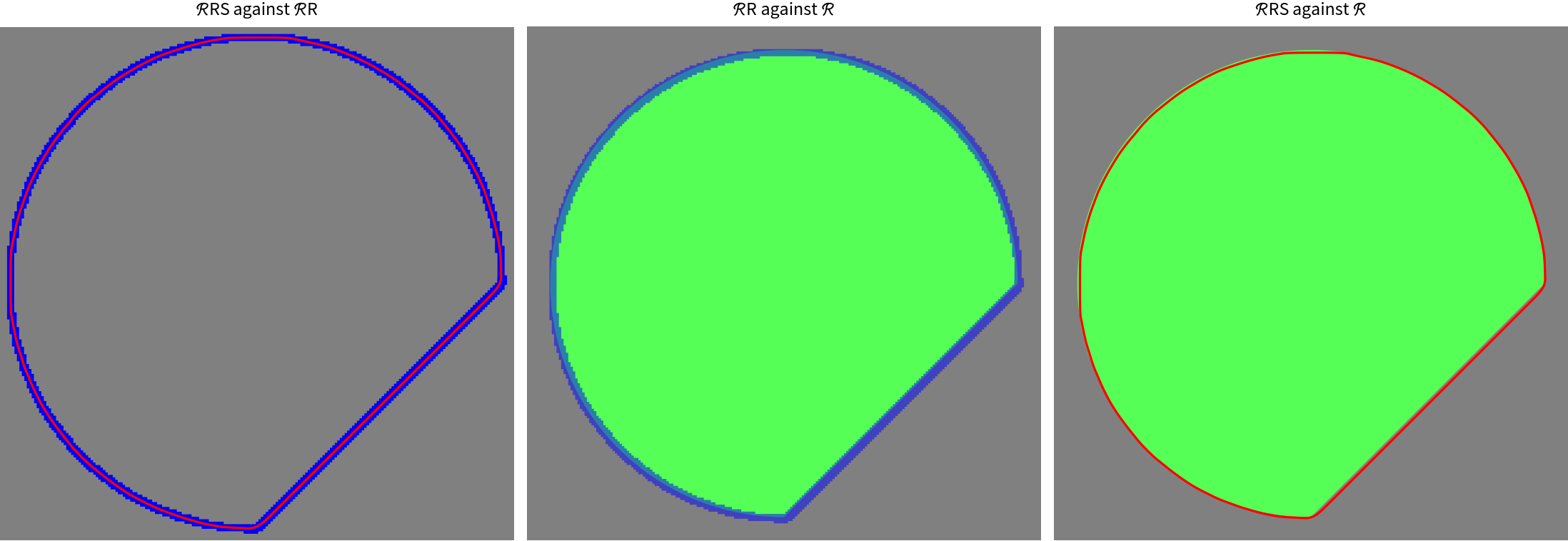
![(* Original exact region *)
\[ScriptCapitalR] = DiskSegment[{110, 110}, 100, {0, 3 Pi/2}];
gr = Graphics[{Lighter@Green, \[ScriptCapitalR]}, PlotRange -> {{0, 220}, {0, 220}}, PlotRangePadding -> None];
img = Rasterize[gr, RasterSize -> {220, 220}];
(* Drop the background component 1, take the contour of the shape *)
contour = ComponentMeasurements[ClusteringComponents[img, 2], "Contours"][[2, 2, 1]];
(* Discretized region with jaggies obtained through Rasterize *)
\[ScriptCapitalR]R = Polygon@First[contour];
(* Parametrize the contour *)
fun = ResourceFunction["CurveToBSplineFunction"][First[contour], 190, "CurveClosed" -> True, "AssignWeights" -> Automatic, "DuplicateNodes" -> (If[Max[#2] > 30, 9, 1] &)];
(* Plot the function with high resolution: we will extract the result of plotting for comparison with NIntegrate *)
plot = ParametricPlot[fun[t], {t, 0, 1}, PlotStyle -> Red, PlotPoints -> 1000, MaxRecursion -> 5];
(* Extract from the plot smoothed version of discretized region \[ScriptCapitalR]2, without jaggies *)
\[ScriptCapitalR]RS = BoundaryDiscretizeGraphics[plot];
(* Calculate the areas *)
Grid[{{"Area of the shape", SpanFromLeft}, {"Exact", "After Rasterize", "From plot", "From NIntegrate"},
{N@Area[\[ScriptCapitalR]], Area[\[ScriptCapitalR]R], Area[\[ScriptCapitalR]RS], Abs@NIntegrate[
Indexed[fun[t], 2] Indexed[D[fun[t], t], 1], {t, 0, 1}]}}, Frame -> All, FrameStyle -> Gray]
(* Visually compare the regions (background is added for better contrast) *)
Grid[{{"\[ScriptCapitalR]RS against \[ScriptCapitalR]R", "\[ScriptCapitalR]R against \[ScriptCapitalR]", "\[ScriptCapitalR]RS against \[ScriptCapitalR]"}, {Show[
Graphics[{AbsoluteThickness[5], Blue, contour}], plot, ImageSize -> 360, Background -> Gray], Show[gr, Graphics[{AbsoluteThickness[5], Blue, Opacity[.5], contour}], ImageSize -> 360, Background -> Gray], Show[gr, plot, ImageSize -> 360, Background -> Gray]}}]](https://www.wolframcloud.com/obj/resourcesystem/images/98f/98f83926-bd08-423a-aa5f-7f67ec1af5b4/7db1efcc03bb193c.png)

![SeedRandom[260];
nodes = RandomPolygon[50][[1]];
funct = ResourceFunction["CurveToBSplineFunction"][nodes, 2, "CurveClosed" -> True][\[FormalT]];
Show[Graphics[{LightGray, Polygon[nodes]}, Frame -> True], ParametricPlot[funct, {\[FormalT], 0, 1}]]](https://www.wolframcloud.com/obj/resourcesystem/images/98f/98f83926-bd08-423a-aa5f-7f67ec1af5b4/11ea665928e6901d.png)
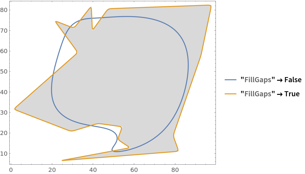
![SeedRandom[1];
nodes = 100 RandomPolygon[17][[1]];
opts = {"FillGaps" -> False, "FillGaps" -> True};
functs = ResourceFunction["CurveToBSplineFunction"][nodes, 12, #, "CurveClosed" -> True][\[FormalT]] & /@ opts;
Show[Graphics[{LightGray, Polygon[nodes]}, Frame -> True],
ParametricPlot[functs, {\[FormalT], 0, 1},
PlotLegends -> (Style[StandardForm@#, "Input", "Notebook", ShowSyntaxStyles -> True] & /@ opts)]]](https://www.wolframcloud.com/obj/resourcesystem/images/98f/98f83926-bd08-423a-aa5f-7f67ec1af5b4/3caf6efc4d95775f.png)
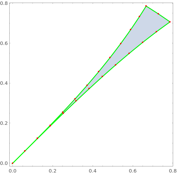
![\[ScriptCapitalR] = ImplicitRegion[
0 < x < 1 && y < Cos[x] && y < Tan[x] && y > Sin[x], {x, y}];
\[ScriptCapitalR]D = BoundaryDiscretizeRegion[\[ScriptCapitalR], MaxCellMeasure -> .1];
nodes = Extract[MeshCoordinates[\[ScriptCapitalR]D], List /@ MeshCells[\[ScriptCapitalR]D, 2][[1, 1]]];
fun = ResourceFunction["CurveToBSplineFunction"][nodes, 2,
"FillGaps" -> False, "DuplicateNodes" -> (If[#3 < \[Pi]/2, 3, 2] &),
"CurveClosed" -> True]
Show[RegionPlot[\[ScriptCapitalR]], ParametricPlot[fun[t], {t, 0, 1}, PlotStyle -> Green], Epilog -> {Red, Point[nodes]}]](https://www.wolframcloud.com/obj/resourcesystem/images/98f/98f83926-bd08-423a-aa5f-7f67ec1af5b4/0706d52aa3f299c7.png)
![Grid[{{"Area of the shape", SpanFromLeft}, {"Exact", "After BoundaryDiscretizeRegion", "From NIntegrate"},
Abs@{N@Area[\[ScriptCapitalR]], Area[\[ScriptCapitalR]D], NIntegrate[Indexed[fun[t], 2] Indexed[D[fun[t], t], 1], {t, 0, 1},
Method -> "LocalAdaptive"]}}, Frame -> All, FrameStyle -> Gray]](https://www.wolframcloud.com/obj/resourcesystem/images/98f/98f83926-bd08-423a-aa5f-7f67ec1af5b4/6bf3c1d686f3257d.png)