Function Repository Resource:

CosDiceLossLayer

Source Notebook

A NetGraph layer implementing cos-dice loss

Contributed by: Michael Sollami

ResourceFunction["CosDiceLossLayer"][q]

represents a net layer that implements cos-dice loss.

Details and Options

ResourceFunction["CosDiceLossLayer"] exposes the following ports for use in NetGraph, etc:
"Input"scalar values between 0 and 1, or arrays of these
"Target"scalar values between 0 and 1, or arrays of these
"Loss"real number
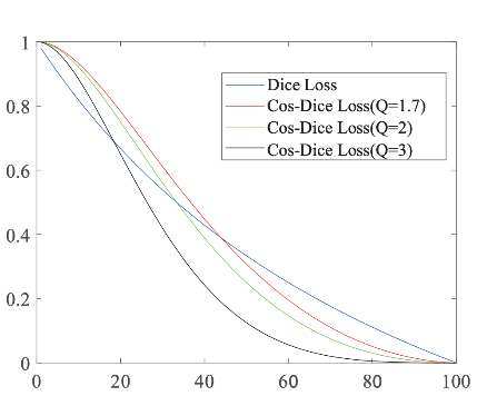
Cos-dice is a variant of the dice coefficient, a popular loss function for medical image segmentation that was defined in Chen et al., "Prostate Segmentation using 2D Bridged U-net", 2018.
The authors provide the following loss-intersection graph, which compares dice loss and cos-dice loss of different q-factors:
ResourceFunction["CosDiceLossLayer"] takes the same options as NetGraph.

Examples

Basic Examples (4) 

Create a cos-dice loss layer:

In[1]:=
loss = ResourceFunction["CosDiceLossLayer"][]
Out[1]=

And apply it to a given input and target:

In[2]:=
loss[<|"Input" -> RandomReal[1, {10, 10}], "Target" -> RandomReal[1, {10, 10}]|>]
Out[2]=

Use CosDiceLossLayer with single probabilities:

In[3]:=
l = ResourceFunction["CosDiceLossLayer"][5, "Input" -> "Scalar"];
l[<|"Input" -> 0.2, "Target" -> 0.8|>]
Out[4]=

Apply CosDiceLossLayer with inputs and targets being matrices of binary class probabilities:

In[5]:=
enc = NetEncoder[{"Image", {6, 11}, ColorSpace -> "Grayscale"}];
loss = ResourceFunction["CosDiceLossLayer"][.25, "Input" -> enc, "Target" -> enc]
Out[6]=

Apply the layer to an input and target:

In[7]:=
loss[<|"Input" -> \!\(\*
GraphicsBox[
TagBox[RasterBox[{{128, 128, 128, 128, 128, 128}, {128, 26, 26, 26, 26, 128}, {128, 26, 26, 26, 26, 128}, {128, 26, 26, 26, 26, 128}, {128, 26, 26, 26, 26, 128}, {128, 128, 128, 128, 128, 128}, {128, 26, 26, 26, 26, 128}, {128, 26, 26, 26, 26, 128}, {128, 26, 26, 26, 26, 128}, {128, 26, 26, 26, 26, 128}, {128, 128, 128, 128, 128, 128}}, {{0, 11}, {6, 0}}, {0, 255},
ColorFunction->GrayLevel],
BoxForm`ImageTag[
       "Byte", ColorSpace -> Automatic, Interleaving -> None, Magnification -> 3],
Selectable->False],
DefaultBaseStyle->"ImageGraphics",
ImageSize->Magnification[3],
ImageSizeRaw->{6, 11},
PlotRange->{{0, 6}, {0, 11}}]\), "Target" -> \!\(\*
GraphicsBox[
TagBox[RasterBox[{{128, 128, 128, 128, 128, 128}, {128, 230, 230, 230,
         230, 128}, {128, 230, 230, 230, 230, 128}, {128, 230, 230, 230, 230, 128}, {128, 230, 230, 230, 230, 128}, {128, 128, 128, 128, 128, 128}, {128, 128, 128, 128, 128, 128}, {128, 128, 128, 128, 128, 128}, {128, 128, 128, 128, 128, 128}, {
        128, 128, 128, 128, 128, 128}, {128, 128, 128, 128, 128, 128}}, {{0, 11}, {6, 0}}, {0, 255},
ColorFunction->GrayLevel],
BoxForm`ImageTag[
       "Byte", ColorSpace -> Automatic, Interleaving -> None, Magnification -> 3],
Selectable->False],
DefaultBaseStyle->"ImageGraphics",
ImageSize->Magnification[3],
ImageSizeRaw->{6, 11},
PlotRange->{{0, 6}, {0, 11}}]\)|>]
Out[7]=

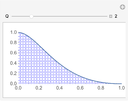
Plot CosDiceLossLayer while varying the q value:

In[8]:=
enc = NetEncoder[{"Image", {64, 64}, "ColorSpace" -> "Grayscale"}];
In[9]:=
Manipulate[
 l = ResourceFunction["CosDiceLossLayer"][q, "Input" -> enc, "Target" -> enc];
 DiscretePlot[
  l[<|"Input" -> Image@ConstantArray[n, {64, 64}], "Target" -> Image@ConstantArray[1, {128, 128}]|>], {n, 0, 1, 0.01}, Joined -> True, Filling -> Axis, FillingStyle -> PatternFilling[{"Octagon", Blue}, ImageScaled[1/40]], PlotRange -> {{0, 1}, {0, 1}}, AspectRatio -> 1/2], {{q, 2, "Q"}, 0.1, 10, .5, Appearance -> "Labeled"}, ControlPlacement -> Top]
Out[9]=

Publisher

Michael Sollami

Version History

  • 1.0.0 – 02 June 2020

Related Resources

License Information