Basic Examples (2)
Define a BinomialDistribution where the probability of success is drawn from a BetaDistribution:
Compute the PDF:
Compute the Mean:
Draw random samples from the distribution. Each sample returns the values of k and p:
Generate multiple samples:
Calculate the LogLikelihood of the samples:
Samples with lower values of k are generally produced by samples with lower values of p:
Scope (2)
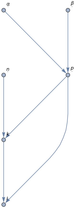
Graph can be used to generate a dependency graph of the individual random variables. Each edge x → y should be read as "x influences y":
The graph is acyclic:
Sample the distribution and compute the expected value. Note that the coordinates are listed in order of appearance of the symbols:
When a ConditionalProductDistribution is defined using unprotected symbols for the bound variables, they will be replaced with symbols of the form x[i]:
Applications (3)
Define a Normal-inverse-Wishart distribution, which is the conjugate prior to a multivariate normal distribution of unknown mean and covariance:
Draw samples from it:
Draw samples from the posterior predictive distribution:
Properties and Relations (3)
A ParameterMixtureDistribution is the marginal distribution of a ConditionalProductDistribution:
Compute the marginal over k by integrating out p from the PDF of the corresponding ConditionalProductDistribution:
The result is the same:
Possible Issues (3)
The distributions need to be ordered correctly and cannot be circular:
In some cases PDF cannot distinguish between evaluating a single coordinate or threading over multiple coordinates. In the following example, the second argument will be interpreted as a pair of coordinates rather than a single 2×2 coordinate:
In this case, wrap the second argument in a list to remove the ambiguity:
Bound variables should not have definitions at the time of defining a ConditionalProductDistribution, since this can have unexpected results:
Use Clear or Block to make sure p has no value at the moment of definition. After that, the variable will have been localized so that p can be used again:
Neat Examples (3)
Define a function that can compute the Expectation of a ConditionalProductDistribution:
Define a distribution using formal symbols (to ensure they do not get renamed) and compute an expected value:
Check the result with a Monte Carlo simulation:
![dist = ResourceFunction[
"ConditionalProductDistribution"][\[FormalK] \[Distributed] BinomialDistribution[10, \[FormalP]], \[FormalP] \[Distributed] BetaDistribution[2, 3]];
SeedRandom[1]; RandomVariate[dist]](https://www.wolframcloud.com/obj/resourcesystem/images/07a/07a341a9-d695-4b4f-b294-1ed39051a921/7e0e47c090a44f0f.png)
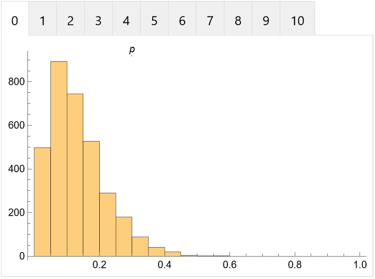
![TabView @ Map[
Histogram[#, {0.05}, PlotRange -> {{0, 1}, All}, ChartLabels -> {Placed[\[FormalP], Above]}] &,
KeySort[GroupBy[RandomVariate[dist, 50000], First -> Last]]
]](https://www.wolframcloud.com/obj/resourcesystem/images/07a/07a341a9-d695-4b4f-b294-1ed39051a921/2cb92583f704b2ae.png)
![dist = ResourceFunction["ConditionalProductDistribution"][
\[FormalL] \[Distributed] GeometricDistribution[\[FormalP]/(\[FormalK] + 1)],
\[FormalK] \[Distributed] BinomialDistribution[\[FormalN], \[FormalP]],
\[FormalP] \[Distributed] BetaDistribution[\[FormalAlpha] + 2, \[FormalBeta] + 2],
{\[FormalN], \[FormalAlpha], \[FormalBeta]} \[Distributed] ProductDistribution[{GeometricDistribution[1/10], 3}]
];
Graph[dist]](https://www.wolframcloud.com/obj/resourcesystem/images/07a/07a341a9-d695-4b4f-b294-1ed39051a921/08f59ebaedcec022.png)
![normalInverseWishartDistribution[\[Mu]0_, \[Lambda]_, \[CapitalPsi]_, \[Nu]_] := ResourceFunction["ConditionalProductDistribution"][
\[FormalMu] \[Distributed] MultinormalDistribution[\[Mu]0, \[FormalCapitalSigma]/\[Lambda]],
\[FormalCapitalSigma] \[Distributed] InverseWishartMatrixDistribution[\[Nu], \[CapitalPsi]]
];](https://www.wolframcloud.com/obj/resourcesystem/images/07a/07a341a9-d695-4b4f-b294-1ed39051a921/2934be4203a32b26.png)

![posteriorPredictiveDistribution[\[Mu]0_, \[Lambda]_, \[CapitalPsi]_, \[Nu]_] := ResourceFunction["ConditionalProductDistribution"][
\[FormalCapitalX] \[Distributed] MultinormalDistribution[\[Mu], \[CapitalSigma]],
{\[Mu], \[CapitalSigma]} \[Distributed] normalInverseWishartDistribution[\[Mu]0, \[Lambda], \[CapitalPsi], \[Nu]]
];
RandomVariate[posteriorPredictiveDistribution[{1, -3}, 5, ( {
{1, 1/2},
{1/2, 2}
} ), 7], 5]](https://www.wolframcloud.com/obj/resourcesystem/images/07a/07a341a9-d695-4b4f-b294-1ed39051a921/457826e8110d09b0.png)

![pdf2 = Simplify@Integrate[
PDF[ResourceFunction[
"ConditionalProductDistribution"][\[FormalK] \[Distributed] BinomialDistribution[n, p], \[FormalP] \[Distributed] BetaDistribution[\[Alpha], \[Beta]]], {k, p}],
{p, 0, 1}
]](https://www.wolframcloud.com/obj/resourcesystem/images/07a/07a341a9-d695-4b4f-b294-1ed39051a921/3ddd9b98e066fafa.png)
![PDF[
ResourceFunction["ConditionalProductDistribution"][
\[FormalX] \[Distributed] ProductDistribution[{NormalDistribution[Indexed[\[FormalY], 1], Indexed[\[FormalY], 2]^2], 2}],
\[FormalY] \[Distributed] ProductDistribution[{NormalDistribution[], 2}]
], {{1, 2}, {3, 4}}]](https://www.wolframcloud.com/obj/resourcesystem/images/07a/07a341a9-d695-4b4f-b294-1ed39051a921/6aa72b324d69da40.png)

![PDF[
ResourceFunction["ConditionalProductDistribution"][
\[FormalX] \[Distributed] ProductDistribution[{NormalDistribution[Indexed[\[FormalY], 1], Indexed[\[FormalY], 2]^2], 2}],
\[FormalY] \[Distributed] ProductDistribution[{NormalDistribution[], 2}]
],
{{{1, 2}, {3, 4}}}
]](https://www.wolframcloud.com/obj/resourcesystem/images/07a/07a341a9-d695-4b4f-b294-1ed39051a921/33a8f7d27ea174e8.png)
![p = 10;
dist = ResourceFunction[
"ConditionalProductDistribution"][\[FormalK] \[Distributed] BinomialDistribution[10, p], p \[Distributed] BetaDistribution[2, 3]]](https://www.wolframcloud.com/obj/resourcesystem/images/07a/07a341a9-d695-4b4f-b294-1ed39051a921/70c0401da328cae2.png)
![Block[{p},
dist = ResourceFunction[
"ConditionalProductDistribution"][\[FormalK] \[Distributed] BinomialDistribution[10, p], p \[Distributed] BetaDistribution[2, 3]]
]](https://www.wolframcloud.com/obj/resourcesystem/images/07a/07a341a9-d695-4b4f-b294-1ed39051a921/734b18cc67b9895e.png)
![conditionalExpectation[expr_, dist_] := Fold[
Expectation[#1, #2] &,
expr,
List @@ dist
];](https://www.wolframcloud.com/obj/resourcesystem/images/07a/07a341a9-d695-4b4f-b294-1ed39051a921/5f03a5361bb54a93.png)
![dist = ResourceFunction[
"ConditionalProductDistribution"][\[FormalK] \[Distributed] BinomialDistribution[n, \[FormalP]], \[FormalP] \[Distributed] BetaDistribution[\[Alpha], \[Beta]]];
conditionalExpectation[\[FormalP]*\[FormalK]^2, dist]](https://www.wolframcloud.com/obj/resourcesystem/images/07a/07a341a9-d695-4b4f-b294-1ed39051a921/1165fd817ae5654b.png)