Wolfram Function Repository
Instant-use add-on functions for the Wolfram Language
Function Repository Resource:
Create an array with a specified slope in the power spectral density
ResourceFunction["ColoredNoise"][count,alpha] creates array of length count with a slope of alpha/2 in the Fourier domain. | |
ResourceFunction["ColoredNoise"][count,name] creates array of length count with a slope corresponding to the name noise color in the Fourier domain. | |
ResourceFunction["ColoredNoise"][{c1,c2,…},alpha] creates a multidimensional array of lengths c1,c2, …. |
Create 10 samples of white noise (slope zero):
| In[1]:= |
| Out[1]= |
Create 10 samples of pink noise (slope minus one):
| In[2]:= |
| Out[2]= |
Create violet noise in two dimensions:
| In[3]:= |
| Out[3]= |  |
Plot different noise slopes in the time domain:
| In[4]:= |
| Out[4]= | 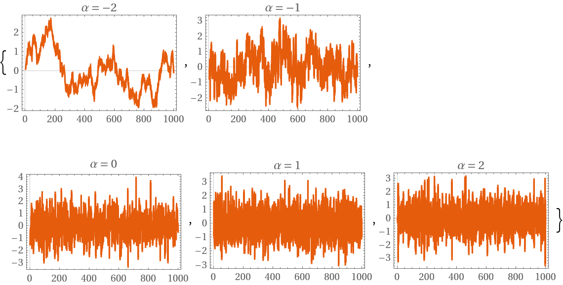 |
Plot different noise slopes in the Fourier domain:
| In[5]:= | ![ListLogLogPlot[
Abs[Fourier[ResourceFunction["ColoredNoise"][10000, #]]][[
2 ;; 5000]], PlotLabel -> ("2\[Cross]Slope = \[Alpha] = " <> ToString[#]), GridLines -> Automatic] & /@ {-2, -1, 0, 1, 2}](https://www.wolframcloud.com/obj/resourcesystem/images/25f/25fbeb21-b28e-42b2-85a2-0cc6b9f5cf34/32a0ad0f5151e5a9.png) |
| Out[5]= | 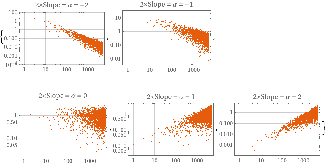 |
Create the same display for two dimensions:
| In[6]:= | ![MatrixPlot[
Log@Abs[Fourier[ResourceFunction["ColoredNoise"][{200, 200}, #]][[
2 ;; 100, 2 ;; 100]]], ColorFunction -> GrayLevel, PlotLabel -> ("\[Alpha] = " <> ToString[#])] & /@ {-2, -1, 0, 1, 2}](https://www.wolframcloud.com/obj/resourcesystem/images/25f/25fbeb21-b28e-42b2-85a2-0cc6b9f5cf34/1d474cb8fc15b4f6.png) |
| Out[6]= | 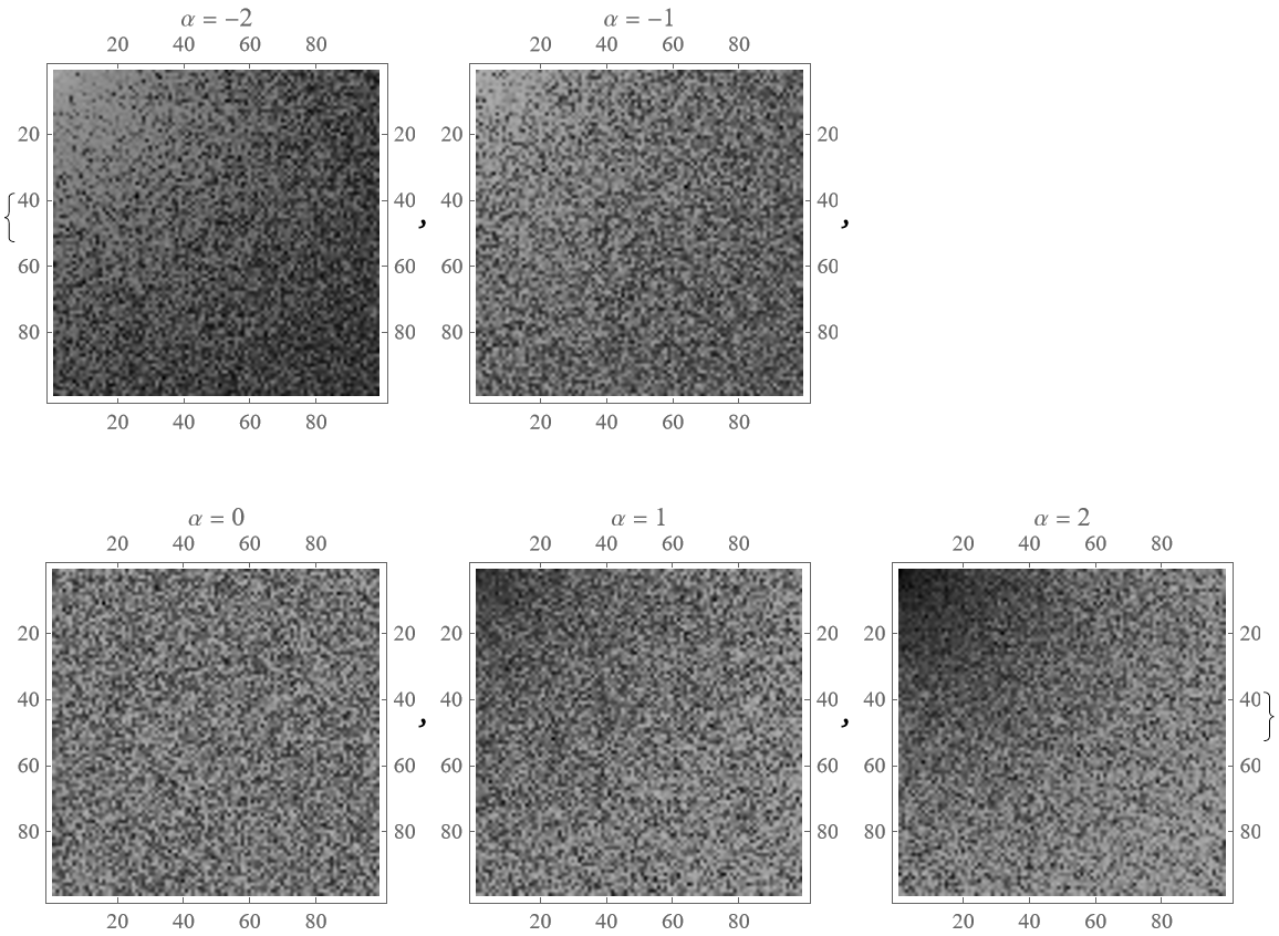 |
All supported color keywords with their respective alpha applied:
| In[7]:= |
| Out[7]= |  |
The mean and standard deviation are always zero and one, respectively:
| In[8]:= |
| Out[8]= |
Turn off the normalization of the standard deviation:
| In[9]:= |
| Out[9]= |
Set the normalization of the standard deviation to a specific value:
| In[10]:= |
| Out[10]= |
Set the offset to a specific value:
| In[12]:= |
| Out[12]= |
Visualize the relation of alphas to the slopes in the power spectral density, the Allan deviation and the influence to the autocorrelation:
| In[13]:= | ![plotOptions = {GridLines -> Automatic, Joined -> True, ImageSize -> 200, PlotStyle -> Black};
Grid[{{"\[Alpha]", "Noise", "Power Spectral Density", "Allan Deviation", "Autocorrelation"}}~Join~
Table[noise = ResourceFunction["ColoredNoise"][10000, alpha]; {alpha,
ListLinePlot[noise, Evaluate[Sequence @@ plotOptions]],
ListLogLogPlot[
ResourceFunction["WelchSpectralEstimate"][noise, 1.0, "Detrend" -> None], Evaluate[Sequence @@ plotOptions]],
ListLogLogPlot[
ResourceFunction["AllanDeviation"][noise, 1.0, {{300}}, "FrequencyData" -> True], Evaluate[Sequence @@ plotOptions], PlotRange -> {{1, Length[noise]/3}, All}],
ListLinePlot[
RotateRight[ListCorrelate[noise, noise, {-1, -1}]/Length[noise], Floor[Length[noise]/2]], Evaluate[Sequence @@ plotOptions], PlotRange -> {All, {-1.05, 1.05}}]
}, {alpha, -2, 2}], Frame -> All]](https://www.wolframcloud.com/obj/resourcesystem/images/25f/25fbeb21-b28e-42b2-85a2-0cc6b9f5cf34/1fa4d8f747c0085e.png) |
| Out[14]= | 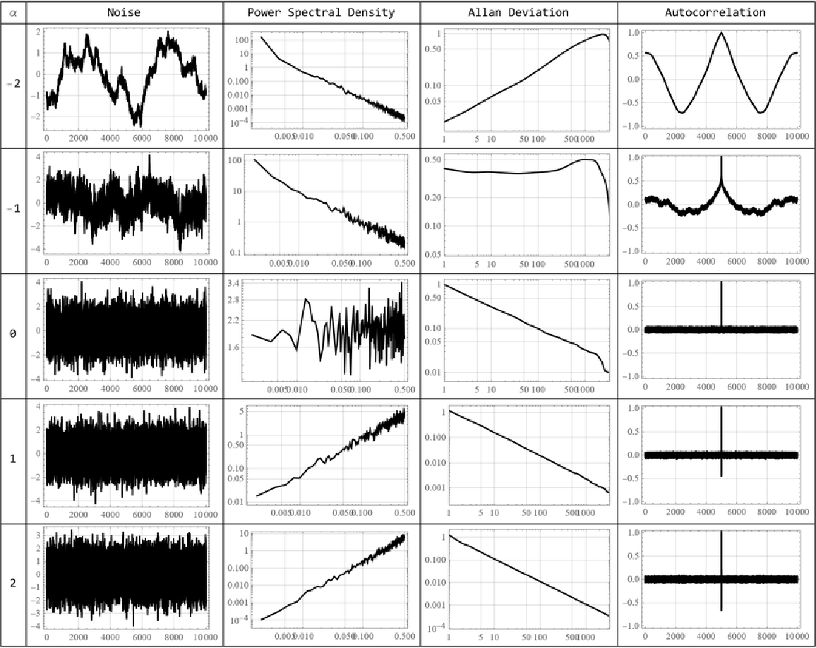 |
Create array with a specified shape of the Allan deviation, mimicking an active atomic clock:
| In[15]:= | ![SeedRandom[314159265];
noise = 5*10^-14*ResourceFunction["ColoredNoise"][10^6, "Blue"] + 10^-14*ResourceFunction["ColoredNoise"][10^6, "Flicker", "Deviation" -> True] + 5*10^-17*
ResourceFunction["ColoredNoise"][10^6, "Red", "Deviation" -> True];
ListLogLogPlot[
ResourceFunction["AllanDeviation"][noise, 1.0, {{300}}, "FrequencyData" -> True], Joined -> True, GridLines -> Automatic, PlotRange -> {{0.5, 3*10^5}, {10^-14, 7*10^-14}}, Epilog -> {Dashed,
Black, InfiniteLine[Log[{{1, 5*10^-14}, {10, 10^-14}}]], Inset["\[Alpha]=1", Log@{1, 2*10^-14}],
Red, InfiniteLine[Log[{{1, 1.2*10^-14}, {10, 1.2*10^-14}}]], Inset["\[Alpha]=-1", Log@{500, 1.5*10^-14}],
Blue, InfiniteLine[Log[{{10^4, 10^-14}, {10^5, 5*10^-14}}]], Inset["\[Alpha]=-2", Log@{5*10^4, 1.5*10^-14}]
}]](https://www.wolframcloud.com/obj/resourcesystem/images/25f/25fbeb21-b28e-42b2-85a2-0cc6b9f5cf34/1702d6f557e97e34.png) |
| Out[17]= | 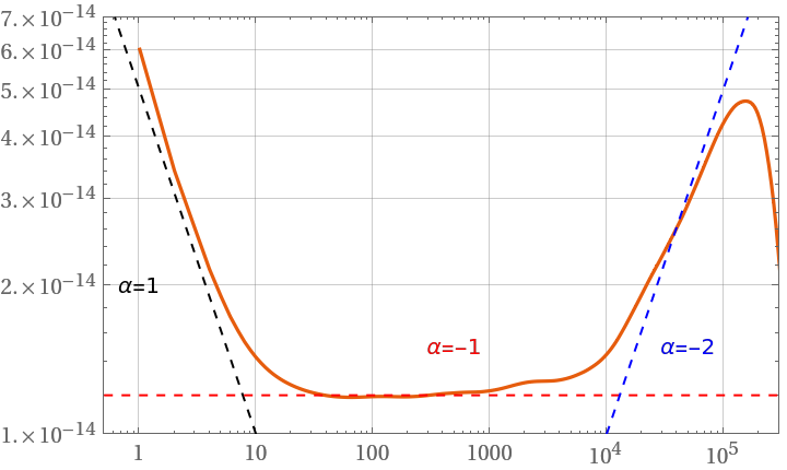 |
The samples argument must be greater than two:
| In[18]:= |
| Out[18]= |  |
The alpha argument must be a known noise color or else a real number:
| In[19]:= |
| Out[19]= |
Noise with alpha values between -1 and -2 sound like a waterfall or turbulent flowing river:
| In[20]:= | ![noise = ResourceFunction["ColoredNoise"][
44100*3, -1]; (*create 3 seconds of noise*)
noise = noise/
Max[Abs[MinMax[noise]]]; (*normalize to [-1,1]*)
ListPlay[noise, SampleRate -> 44100]](https://www.wolframcloud.com/obj/resourcesystem/images/25f/25fbeb21-b28e-42b2-85a2-0cc6b9f5cf34/11dabe570868c421.png) |
| Out[21]= | 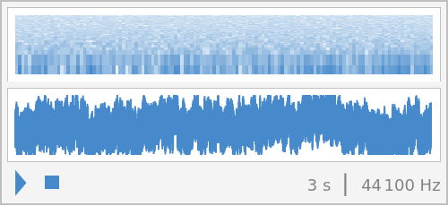 |
Create soft 2D-noise maps by choosing low alpha values:
| In[22]:= |
| Out[22]= | 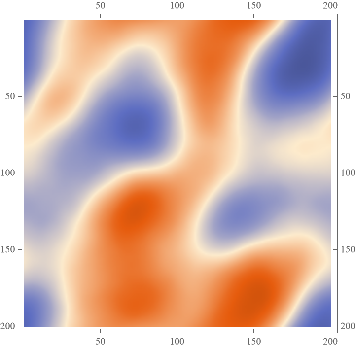 |
This work is licensed under a Creative Commons Attribution 4.0 International License