Wolfram Function Repository
Instant-use add-on functions for the Wolfram Language
Function Repository Resource:
Make a histogram of the heights in a clustering tree
ResourceFunction["ClusteringTreeHeightHistogram"][tree] plots a histogram of the cluster heights in the ClusteringTree tree. | |
ResourceFunction["ClusteringTreeHeightHistogram"][tree,bspec] plots a histogram with bin width specification bspec. | |
ResourceFunction["ClusteringTreeHeightHistogram"][tree,bspec,hspec] plots a histogram with bin heights computed according to the specification hspec. |
Obtain a cluster hierarchy from a list of numbers:
| In[1]:= |
| In[2]:= |
| Out[2]= | 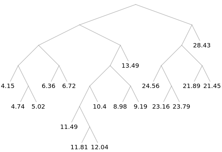 |
Plot the histogram of heights at which the clusters merge:
| In[3]:= |
| Out[3]= | 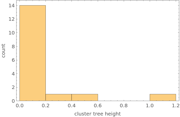 |
Make a list of data:
| In[7]:= | ![cities = {Entity["City", {"Sydney", "NewSouthWales", "Australia"}], Entity["City", {"Melbourne", "Victoria", "Australia"}], Entity["City", {"Brisbane", "Queensland", "Australia"}], Entity["City", {"Perth", "WesternAustralia", "Australia"}], Entity["City", {"Adelaide", "SouthAustralia", "Australia"}], Entity["City", {"GoldCoast", "Queensland", "Australia"}], Entity["City", {"Newcastle", "NewSouthWales", "Australia"}], Entity["City", {"Canberra", "AustralianCapitalTerritory", "Australia"}], Entity["City", {"SunshineCoast", "Queensland", "Australia"}], Entity["City", {"Wollongong", "NewSouthWales", "Australia"}], Entity["City", {"Blacktown", "NewSouthWales", "Australia"}], Entity["City", {"Hobart", "Tasmania", "Australia"}], Entity["City", {"CityOfStirling", "WesternAustralia", "Australia"}], Entity["City", {"Geelong", "Victoria", "Australia"}], Entity["City", {"Townsville", "Queensland", "Australia"}], Entity["City", {"Gosford", "NewSouthWales", "Australia"}], Entity["City", {"Ipswich", "Queensland", "Australia"}], Entity["City", {"Cairns", "Queensland", "Australia"}], Entity["City", {"Toowoomba", "Queensland", "Australia"}], Entity["City", {"Darwin", "NorthernTerritory", "Australia"}], Entity["City", {"Launceston", "Tasmania", "Australia"}]};](https://www.wolframcloud.com/obj/resourcesystem/images/6d9/6d9a33d7-3612-4fe9-863d-275321542e17/2db19bd944ec8f4c.png) |
Compute the clustering tree:
| In[8]:= |
| Out[8]= | 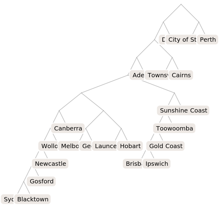 |
Plot the histogram of heights to help choose a height at which to cut the tree:
| In[9]:= |
| Out[9]= | 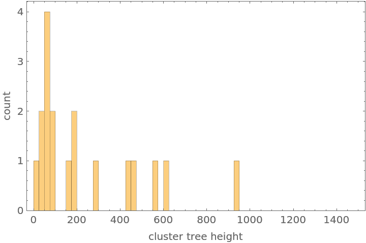 |
Plot the dendrogram to help choose a height at which to cut the tree:
| In[10]:= |
| Out[10]= | 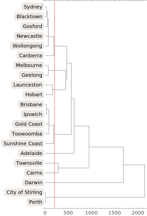 |
Extract the clusters at a height of 200:
| In[11]:= |
| Out[11]= |  |
Plot the locations of the cites colored by cluster:
| In[12]:= | ![Graphics[{LightGray, CountryData["Australia", "Polygon"], MapThread[{cluster, color} |-> ({PointSize[Large], color, Tooltip[Point[Reverse[CityData[#, "Coordinates"]]], CityData[#, "Name"]]} & /@ cluster), {clusters, ColorData[97] /@ Range@Length@clusters}]}]](https://www.wolframcloud.com/obj/resourcesystem/images/6d9/6d9a33d7-3612-4fe9-863d-275321542e17/2f6cd529b9d3abb0.png) |
| Out[12]= | 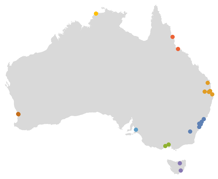 |
Wolfram Language 13.0 (December 2021) or above
This work is licensed under a Creative Commons Attribution 4.0 International License