Wolfram Function Repository
Instant-use add-on functions for the Wolfram Language
Function Repository Resource:
Produce Chebyshev nodes
ResourceFunction["ChebyshevNodes"][n] produces n Chebyshev nodes in the range from -1 to 1. | |
ResourceFunction["ChebyshevNodes"][n,{min,max}] produces n Chebyshev nodes in the domain min to max. |
Create ten Chebyshev nodes analytically:
| In[1]:= |
| Out[1]= |
Approximate the numbers:
| In[2]:= |
| Out[2]= |
Create the numbers on a domain from 0 to 2π:
| In[3]:= |
| Out[3]= |  |
Show on a number line:
| In[4]:= |
| Out[4]= |
Find points for fifth order approximation:
| In[5]:= | ![n = 5;
min = 0.0;
max = Pi;
x =.;
pts = ResourceFunction["ChebyshevNodes"][n + 1, {min, max}]](https://www.wolframcloud.com/obj/resourcesystem/images/57e/57eb7966-1326-447f-8083-df78fe003c4e/03527d29335f9e37.png) |
| Out[6]= |
Perform the approximation of Cos[x]:
| In[7]:= |
| Out[8]= |
Represent the approximation as a polynomial:
| In[9]:= |
| Out[9]= |
Compare the functions:
| In[10]:= |
| Out[10]= | 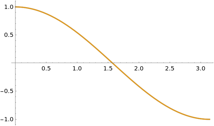 |
Show the difference:
| In[11]:= |
| Out[11]= | 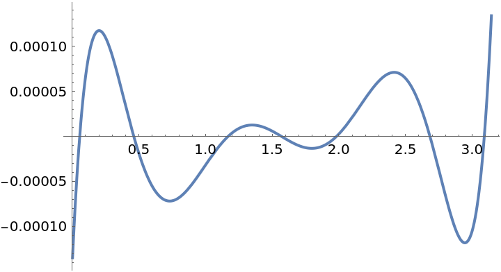 |
Compare to the error from a fifth-order series expansion evaluated at the midpoint:
| In[12]:= |
| Out[12]= | 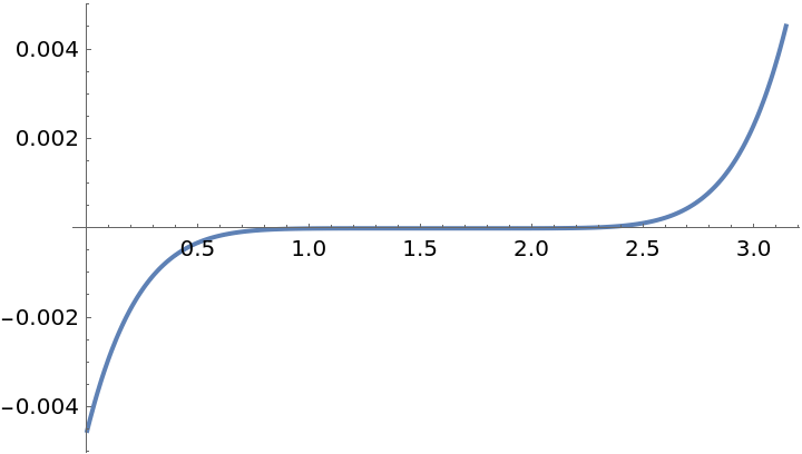 |
The Chebyshev nodes are related to the roots of Chebyshev polynomials of the first kind:
| In[13]:= |
| Out[14]= | 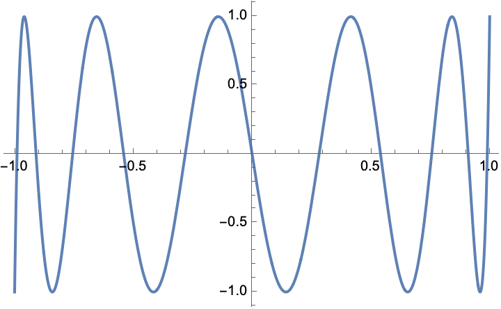 |
Compare the zeros by finding the roots numerically and using the function ChebyshevNodes:
| In[15]:= | ![a = Sort[
DeleteDuplicates[
Identity[x /. FindRoot[f, {x, #}] & /@ Subdivide[-1, 1, 30]], Abs[#1 - #2] < 10^-4 &]];
b = ResourceFunction["ChebyshevNodes"][11];
Chop[a - b]](https://www.wolframcloud.com/obj/resourcesystem/images/57e/57eb7966-1326-447f-8083-df78fe003c4e/47377f463112095e.png) |
| Out[16]= |
Chebyshev nodes match the coordinate components of CirclePoints:
| In[17]:= |
| Out[17]= |
Show how Chebyshev nodes are related to equi-distantly spaced points on a semi-circle:
| In[18]:= | ![n = 10;
cns = ResourceFunction["ChebyshevNodes"][n];
p1 = AngleVector /@ MovingAverage[Subdivide[Pi, 0, n], 2];
p2 = {#, 0} & /@ cns;
Graphics[{
Style[Circle[{0, 0}, 1, {0, Pi}], Black],
Style[MapThread[Arrow[{#1, #2}] &, {p1, p2}], Black],
Style[Disk[p1, 0.02], Blue],
Style[Disk[p2, 0.02], Red],
Style[InfiniteLine[{{-1, 0}, {1, 0}}]]
},
PlotRange -> {{-1.25, 1.25}, {-0.25, 1.25}}
]](https://www.wolframcloud.com/obj/resourcesystem/images/57e/57eb7966-1326-447f-8083-df78fe003c4e/7ff2d792947d8c95.png) |
| Out[19]= | 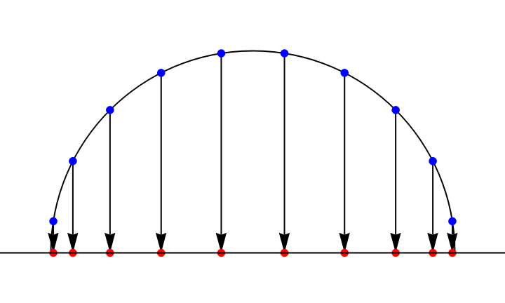 |
Wolfram Language 13.0 (December 2021) or above
This work is licensed under a Creative Commons Attribution 4.0 International License