Wolfram Function Repository
Instant-use add-on functions for the Wolfram Language
Function Repository Resource:
Evaluate Bulirsch's general complete elliptic integral
ResourceFunction["BulirschCEL"][m,p,a,b] gives Bulirsch's general complete elliptic integral |
Evaluate numerically:
| In[1]:= |
|
| Out[1]= |
|
Evaluate numerically for complex arguments:
| In[2]:= |
|
| Out[2]= |
|
Evaluate to high precision:
| In[3]:= |
|
| Out[3]= |
|
The precision of the output tracks the precision of the input:
| In[4]:= |
|
| Out[4]= |
|
Simple exact results are generated automatically:
| In[5]:= |
|
| Out[5]= |
|
| In[6]:= |
|
| Out[6]= |
|
BulirschCEL threads elementwise over lists:
| In[7]:= |
|
| Out[7]= |
|
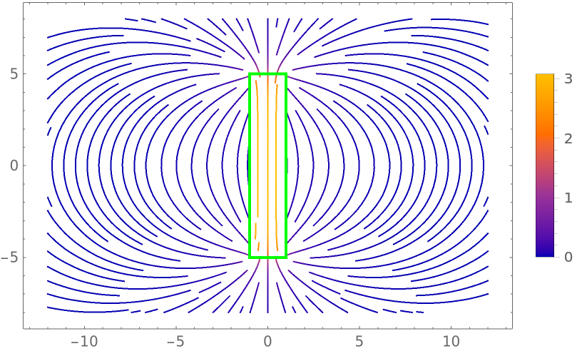
Evaluate the mutual inductance of two coaxial circles:
| In[8]:= |
![With[{a = Quantity[2, "Centimeters"], b = Quantity[3, "Centimeters"], h = Quantity[11, "Centimeters"]},
UnitConvert[
Sqrt[(a - b)^2 + h^2]
ResourceFunction[
"BulirschCEL"][((a + b)^2 + h^2)/((a - b)^2 + h^2), 1, (
2 a b)/((a - b)^2 + h^2), -((2 a b)/((a - b)^2 + h^2))] Quantity[
"MagneticConstant"], "Henries"]]](https://www.wolframcloud.com/obj/resourcesystem/images/d42/d42f70f3-2dd9-4099-8711-7b63ee5e1048/5589425e287d39d9.png)
|
| Out[8]= |
|
Compare with the result of NIntegrate:
| In[9]:= |
![With[{a = Quantity[2, "Centimeters"], b = Quantity[3, "Centimeters"], h = Quantity[11, "Centimeters"]},
UnitConvert[(a b)/
2 NIntegrate[Cos[\[Theta]]/Sqrt[
h^2 + a^2 + b^2 - 2 a b Cos[\[Theta]]], {\[Theta], 0, 2 \[Pi]}, WorkingPrecision -> 25] Quantity["MagneticConstant"], "Henries"]]](https://www.wolframcloud.com/obj/resourcesystem/images/d42/d42f70f3-2dd9-4099-8711-7b63ee5e1048/3261a268cbeb130e.png)
|
| Out[9]= |
|
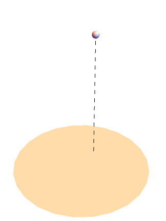
Visualize the solid angle subtended by a circular disk:
| In[10]:= |
![With[{L = 2, r0 = 2/5, rm = 1},
Graphics3D[{EdgeForm[], Polygon[PadRight[N@CirclePoints[rm, 24], {Automatic, 3}]], {Dashed,
Line[{{r0, 0, 0}, {r0, 0, L}}]}, Sphere[{r0, 0, L}, rm/20]}, Boxed -> False, ViewPoint -> {-2.4, -1.3, 2.}]]](https://www.wolframcloud.com/obj/resourcesystem/images/d42/d42f70f3-2dd9-4099-8711-7b63ee5e1048/0a1d879852ad83f1.png)
|
| Out[10]= |
|
Evaluate the solid angle:
| In[11]:= |
![With[{L = 2, r0 = 2/5, rm = 1}, N[2 \[Pi] Boole[r0 < rm] - (
4 L rm)/((rm - r0) Sqrt[L^2 + (rm - r0)^2])
ResourceFunction["BulirschCEL"][(L^2 + (rm + r0)^2)/(
L^2 + (rm - r0)^2), ((rm + r0)/(rm - r0))^2, 1, (rm + r0)/(
rm - r0)], 20]]](https://www.wolframcloud.com/obj/resourcesystem/images/d42/d42f70f3-2dd9-4099-8711-7b63ee5e1048/4d41afdf1149c6f7.png)
|
| Out[11]= |
|
Compare with the result of NIntegrate:
| In[12]:= |
|
| Out[12]= |
|
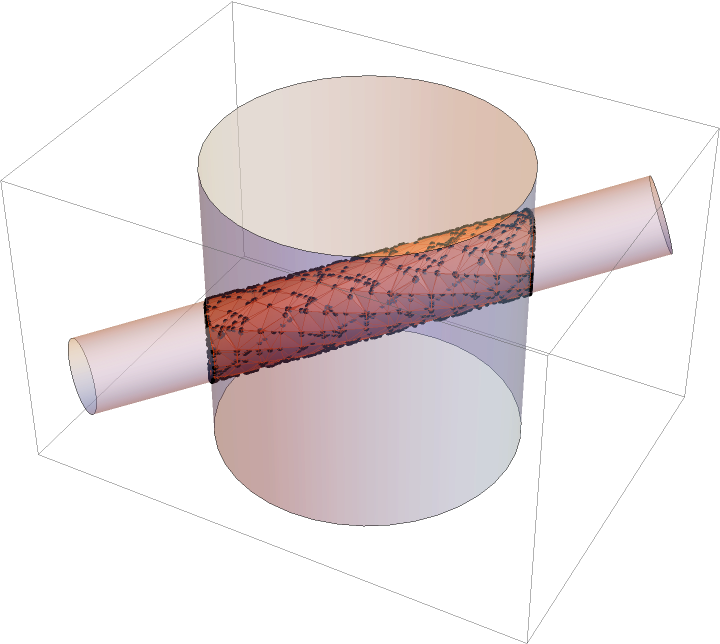
Visualize the intersection of two cylinders:
| In[13]:= |
![With[{r1 = 1/4, r2 = 1}, Show[{Graphics3D[{Opacity[0.4], Cylinder[{{-3/2, -1, -1/2}, {3/2, 1, 1/2}}, r1], Cylinder[{{0, 0, -1}, {0, 0, 1}}, r2]}], Region[RegionIntersection[
Cylinder[{{-3/2, -1, -1/2}, {3/2, 1, 1/2}}, r1], Cylinder[{{0, 0, -1}, {0, 0, 1}}, r2]], PlotTheme -> "Web"]}]]](https://www.wolframcloud.com/obj/resourcesystem/images/d42/d42f70f3-2dd9-4099-8711-7b63ee5e1048/2ccc76d67544472f.png)
|
| Out[13]= |
|
Compute the volume of the intersection of two cylinders:
| In[14]:= |
![With[{r1 = 1/4, r2 = 1, \[Beta] = VectorAngle[{3/2, 1, 1/2}, {0, 0, 1}]}, N[(8 r2^3)/
3 Csc[\[Beta]] ResourceFunction["BulirschCEL"][1 - (r1/r2)^2, 1, 2 (r1/r2)^2, (r1/r2)^2 (1 - (r1/r2)^2)], 20]]](https://www.wolframcloud.com/obj/resourcesystem/images/d42/d42f70f3-2dd9-4099-8711-7b63ee5e1048/6d94bea4f9363db0.png)
|
| Out[14]= |
|
Compare with the result of Volume:
| In[15]:= |
![With[{r1 = 1/4, r2 = 1}, Volume[RegionIntersection[
Cylinder[{{-3/2, -1, -1/2}, {3/2, 1, 1/2}}, r1], Cylinder[{{0, 0, -1}, {0, 0, 1}}, r2]], WorkingPrecision -> 20]]](https://www.wolframcloud.com/obj/resourcesystem/images/d42/d42f70f3-2dd9-4099-8711-7b63ee5e1048/3a7de40f0b2a3cc8.png)
|
| Out[15]= |
|
Complete Legendre-Jacobi elliptic integrals of all three kinds can be expressed in terms of BulirschCEL:
| In[16]:= |
|
| Out[16]= |
|
| In[17]:= |
|
| Out[17]= |
|
| In[18]:= |
|
| Out[18]= |
|
BulirschCEL can be used to represent linear combinations of complete elliptic integrals:
| In[19]:= |
![With[{a = 4, b = 5, m = 2/3}, N[{a EllipticK[m] + b EllipticE[m], ResourceFunction["BulirschCEL"][1 - m, 1, a + b, a + b (1 - m)]}]]](https://www.wolframcloud.com/obj/resourcesystem/images/d42/d42f70f3-2dd9-4099-8711-7b63ee5e1048/71b74121a17faa2b.png)
|
| Out[19]= |
|
| In[20]:= |
![With[{a = 4, b = 5, n = -1/8, m = 2/3}, N[{a EllipticK[m] + b EllipticPi[n, m], ResourceFunction["BulirschCEL"][1 - m, 1 - n, a + b, a (1 - n) + b]}]]](https://www.wolframcloud.com/obj/resourcesystem/images/d42/d42f70f3-2dd9-4099-8711-7b63ee5e1048/69411ef6f28714f9.png)
|
| Out[20]= |
|
JacobiZeta can be expressed in terms of BulirschCEL:
| In[21]:= |
![With[{\[Phi] = 2, m = 1/3}, N[{JacobiZeta[\[Phi], m], (m Sin[2 \[Phi]])/
2 ResourceFunction["BulirschCEL"][1 - m, 1 - m Sin[\[Phi]]^2, 0, Sqrt[1 - m Sin[\[Phi]]^2]]/
ResourceFunction["BulirschCEL"][1 - m, 1, 1, 1]}]]](https://www.wolframcloud.com/obj/resourcesystem/images/d42/d42f70f3-2dd9-4099-8711-7b63ee5e1048/553e143bfc870741.png)
|
| Out[21]= |
|
Wolfram Language 12.3 (May 2021) or above
This work is licensed under a Creative Commons Attribution 4.0 International License
![(* Evaluate this cell to get the example input *) CloudGet["https://www.wolframcloud.com/obj/cec60d94-f28a-4e80-944e-c04ba360be71"]](https://www.wolframcloud.com/obj/resourcesystem/images/d42/d42f70f3-2dd9-4099-8711-7b63ee5e1048/6767f4d58a8890b1.png)