Wolfram Function Repository
Instant-use add-on functions for the Wolfram Language
Function Repository Resource:
Create a graph of an order-n buckyball
ResourceFunction["BuckyballGraph"][n] gives a graph corresponding to an order-n buckyball. | |
ResourceFunction["BuckyballGraph"][class,n] gives a graph corresponding to an order-n buckyball of class class. |
Generate an order-2 buckyball:
| In[1]:= |
| Out[1]= | 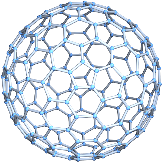 |
The above buckyball is a class II, order-2 buckyball:
| In[2]:= |
| Out[2]= | 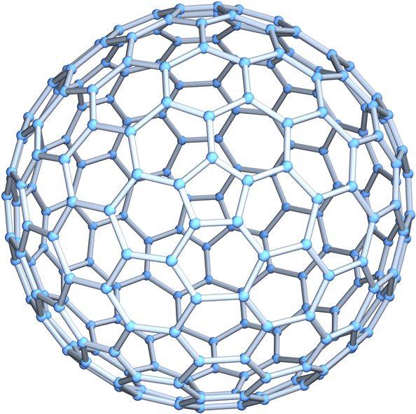 |
Generate a class I, order-3 buckyball:
| In[3]:= |
| Out[3]= | 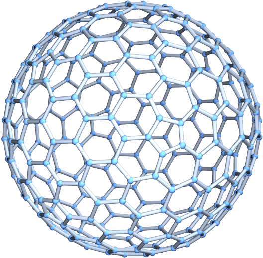 |
Generate an order-2 buckyball with specially computed coordinates:
| In[4]:= |
| Out[4]= | 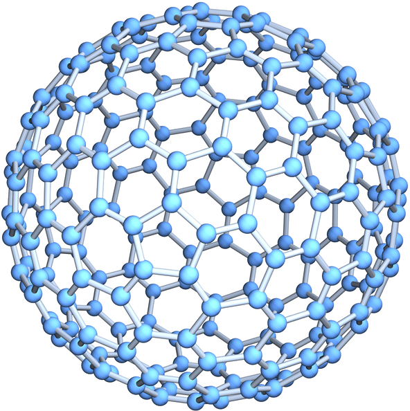 |
Generate a dodecahedral graph:
| In[5]:= |
| Out[5]= | 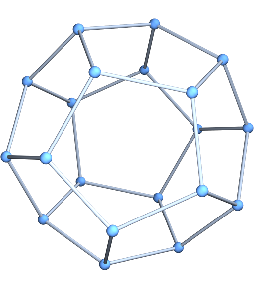 |
Show an order-1 buckyball of different classes:
| In[6]:= | ![Table[ResourceFunction["BuckyballGraph"][class, 1, PlotLabel -> "Class " <> IntegerString[class], VertexCoordinates -> "Embedded"], {class, 1, 2}] // GraphicsRow](https://www.wolframcloud.com/obj/resourcesystem/images/639/6398678f-3a81-4002-b571-4ab55390f437/03c28b2b162a8193.png) |
| Out[6]= |  |
Convert to a Graph object:
| In[7]:= |
| Out[7]= | 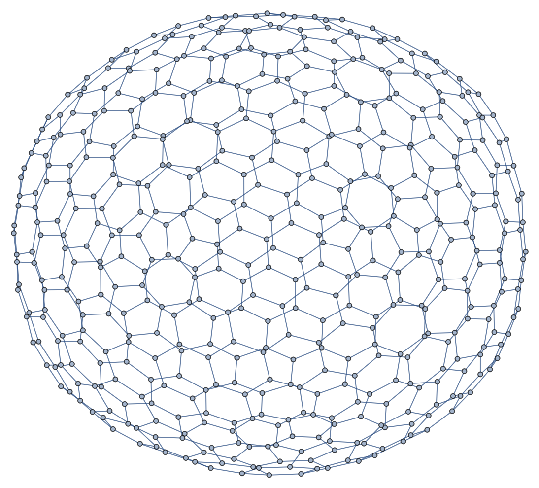 |
Specify various layouts for the buckyball graph:
| In[8]:= |
| Out[8]= | 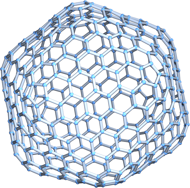 |
| In[9]:= |
| Out[9]= | 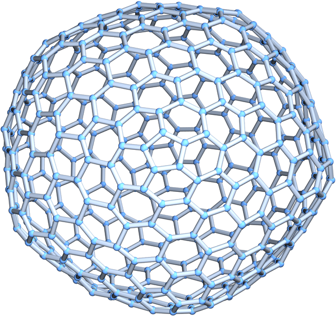 |
Use a large graph theme:
| In[10]:= |
| Out[10]= | 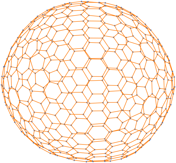 |
By default, vertex coordinates are computed automatically, depending on the setting for GraphLayout:
| In[11]:= |
| Out[11]= | 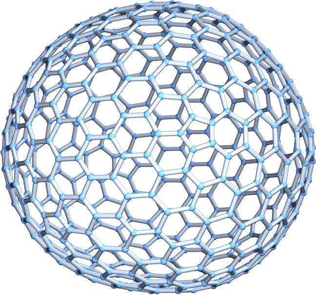 |
Use specially computed coordinates for the vertices:
| In[12]:= |
| Out[12]= | 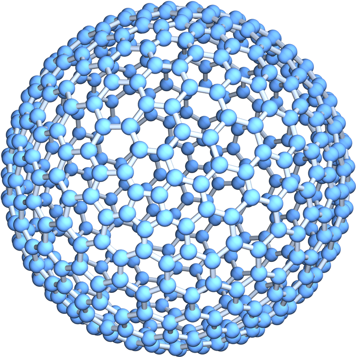 |
BuckyballGraph[1] (the class II, order-1 buckyball) is the graph corresponding to the truncated icosahedron:
| In[13]:= |
| Out[13]= | 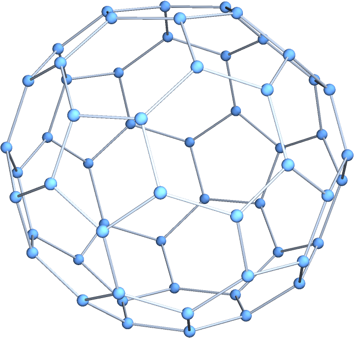 |
| In[14]:= |
| Out[14]= |
Generate a fullerene molecule from its corresponding skeletal graph:
| In[15]:= | ![bucky = ResourceFunction["BuckyballGraph"][1, 2];
el = EdgeList[bucky];
dbl = FindIndependentEdgeSet[bucky];
bmol = MoleculeModify[
Molecule[ConstantArray[Atom["C"], VertexCount[bucky]], Join[Bond[{##}, "Single"] & @@@ Complement[el, dbl], Bond[{##}, "Double"] & @@@ dbl], AtomCoordinates -> QuantityArray[1.6 GraphEmbedding[bucky], "Angstroms"]], "EnergyMinimizeAtomCoordinates"]](https://www.wolframcloud.com/obj/resourcesystem/images/639/6398678f-3a81-4002-b571-4ab55390f437/01e61512f2e42d56.png) |
| Out[16]= |
Visualize the graph and the corresponding fullerene:
| In[17]:= |
| Out[17]= | 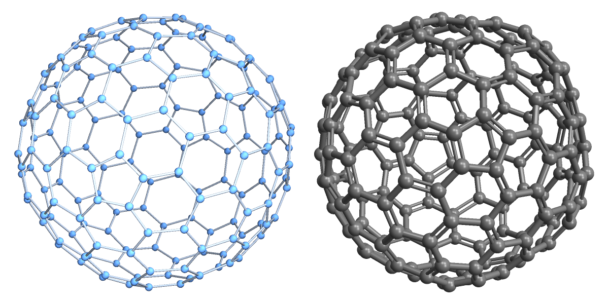 |
This work is licensed under a Creative Commons Attribution 4.0 International License