Basic Examples (2) 

Find the eigenvalues of myoglobin:

In[1]:=

Out[2]=

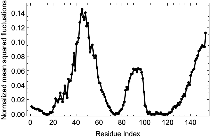
Visualize the fluctuations in the second mode (slowest possible non-trivial mode):

In[3]:=

Out[4]=

Scope (6) 

BioMoleculeResidueFluctuations can accept a BioMolecule as an input:

In[5]:=

See the keys available in the result:

In[6]:=

Out[6]=

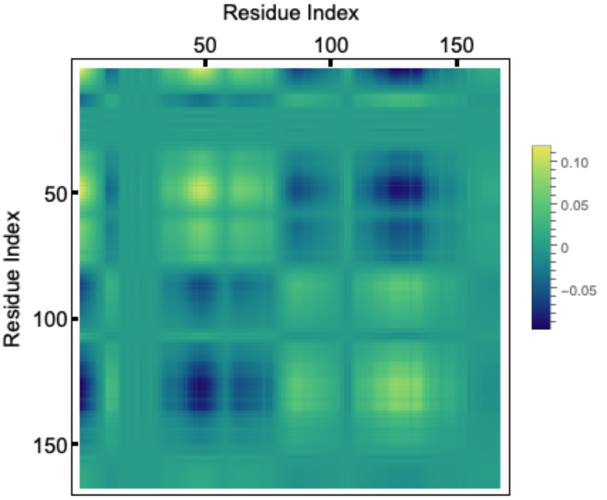
Display a correlation matrix of deviations in the human KRAS G12C mutant for the slowest mode constructed using the "Eigenvectors" and "Eigenvalues":

In[7]:=

Out[8]=

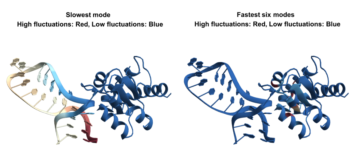
BioMoleculeResidueFluctuations can analyze nucleic acid structures and protein-nucleic acid complexes too. Here is the visualization of the "NormalizedMeanSquaredFluctuations" in slow and fast modes for a protein-RNA complex:

In[9]:=

Out[17]=

Fluctuations of folded structures from an amino acid sequence can also be computed:

In[18]:=

Out[22]=

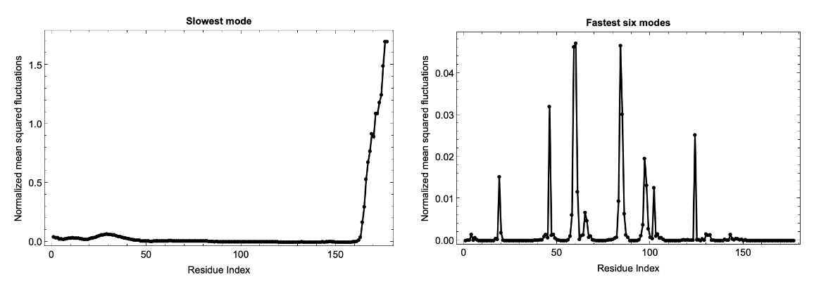
Analysis of computationally predicted structures in the AlphaFold Protein Structure Database can be performed by providing the relevant UniProt ID using the ExternalIdentifier:

In[23]:=

Out[24]=

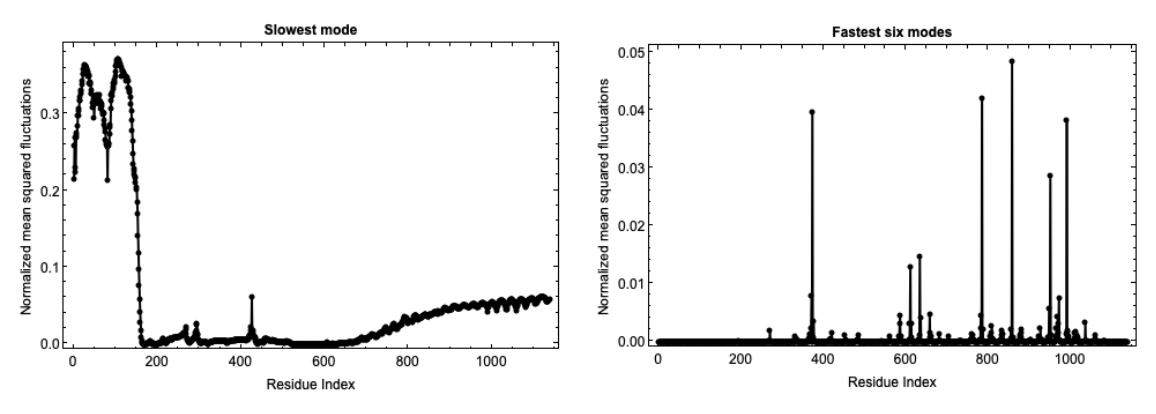
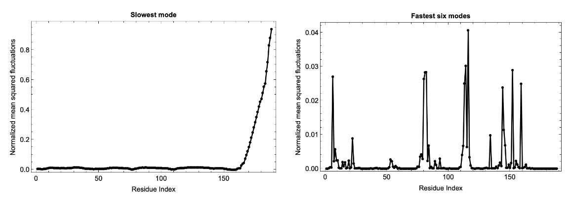
Fluctuations of isoforms in the predicted structures of the AlphaFold Database can also be computed:

In[25]:=

Out[26]=

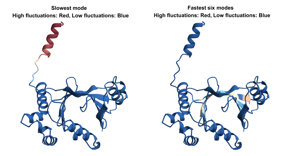
Fluctuations of predicted structures from the ESM Metagenomic Atlas can also be computed using the MGnify Protein ID:

In[27]:=

Out[28]=

Applications (6) 

Let us analyze the mean squared fluctuations in HIV-1 protease:

In[29]:=

In[30]:=

Out[30]=

Since the "Eigenvalues" are sorted in ascending order let us get the lowest five eigenvalues:

In[31]:=

Out[31]=

The lowest eigenvalue is much much smaller than the others and close to zero and it does not return any meaningful variation in the fluctuations. So the slowest mode (smallest eigenvalue) for which we can see meaningful patterns in the fluctuation is k=2:

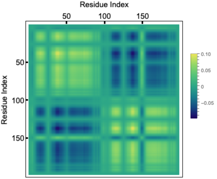
If we take the outer-product of an eigenvector corresponding to a given mode and divide it by the eigenvalue, the diagonal elements represent the residue fluctuations and the off diagonal elements represents correlations. Let us visualize the correlation matrix for the slowest mode. The colorbar indicates normalized mean squared fluctuations:

In[32]:=

Out[33]=

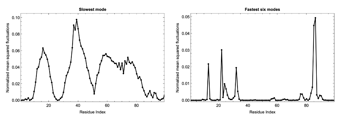
HIV-1 protease is a dimer and the fluctuations for two chains (99 residues each) follows identical pattern, as can be seen in the correlation matrix. Here we plot the fluctuation for a single chain for both the slowest mode (left) and fastest six modes combined (right). Usually the fastest mode (largest eigenvalue) has very sharp peaks, so to see the average fluctuation, we combine the fastest six modes:

In[34]:=

Out[35]=

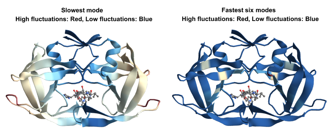
Let us visualize the fluctuations for the slowest and fastest modes on the structure. For the slow modes the minima of fluctuations (in blue) corresponds to hinge regions which plays important functions in the protein and the maxima (in red) represents regions of highest mobility. For the fastest modes, the large fluctuation region (in red), plays a key role in the stability of the protein:

In[36]:=

Out[37]=

Options (2) 

CutOff (2) 

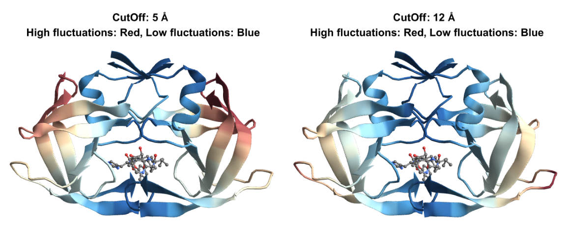
Set a custom "CutOff" distance within which inter-residue interactions will be taken into account:

In[38]:=

Visualize the fluctuations for both cutoffs in the slowest mode:

In[39]:=

Out[40]=

Neat Examples (2) 

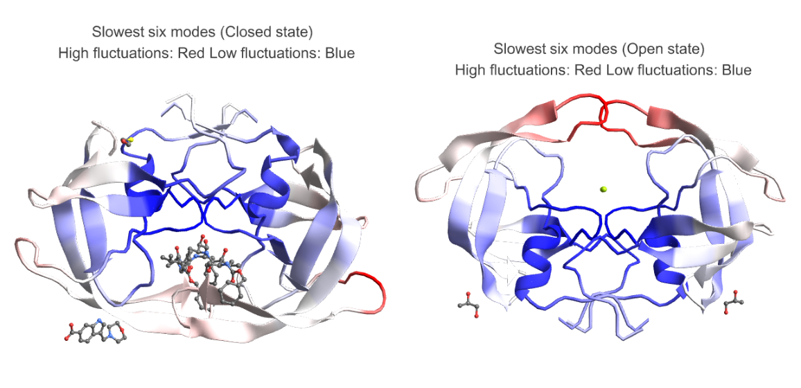
We analyze the average fluctuations in the slowest six modes of HIV-1 protease in open (PDB ID - 2PC0) and closed state (PDB ID - 4TVH):

In[41]:=

In[42]:=

The plots below highlight the motion in the flap area in open state (right) and lack thereof in closed state (left) which is very similar to an existing study of molecular dynamics simulation of HIV-1 protease[2]:

In[43]:=

Out[44]=