Wolfram Function Repository
Instant-use add-on functions for the Wolfram Language
Function Repository Resource:
Compute the Barnes multiple gamma function numerically
ResourceFunction["BarnesMultipleGamma"][w,{a1,...,an}] gives Γn(w❘a1,…,an). |


Evaluate numerically:
| In[1]:= | 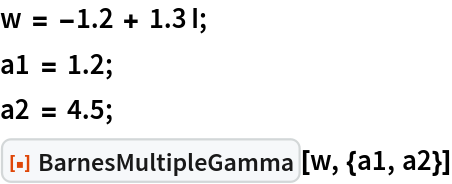 |
| Out[4]= |  |
BarnesMultipleGamma supports arbitrary integer orders subject to limits in computing accuracy:
| In[5]:= |  |
| Out[5]= |  |
The Barnes multiple gamma function can be used to define the double sine function:
| In[6]:= |  |
| Out[7]= |  |
If the order is zero then Γ0(w) = 1/w:
| In[8]:= | 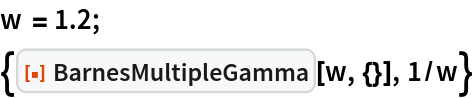 |
| Out[9]= |  |
If the order is one then Γ1 is related to the usual gamma function Γ1(w❘a)=ⅇ(w/a - 1/2) log aΓ(w/a)(2 π)-1/2:
| In[10]:= |  |
| Out[12]= |  |
If the order is two and a1=a2=1 then Γ2 is related to the Barnes G function, Γ2(w❘1,1)=ⅇ(w/2 - 1/2) log (2 π)eζ′(-1)G(w)-1:
| In[13]:= |  |
| Out[14]= |  |
BarnesMultipleGamma satisfies a recurrence relation:
| In[15]:= |  |
| Out[18]= |  |
The parameters should be strictly positive real numbers:
| In[19]:= |  |
| Out[19]= |  |
The recurrence method in use can lead to exceeding recursion depth limitations:
| In[20]:= |  |
| Out[20]= |  |
BarnesMultipleGamma does not compute exact values even when input is exact:
| In[21]:= |  |
| Out[21]= |  |
For special values of the parameters one can often calculate closed form expressions involving the Hurwitz zeta function:
| In[22]:= | ![BarnesGamma123[w_] := Module[{b = {3, 4, 5, 6, 7, 8}, c = {1, 1, 2, 3, 4, 5}, q, B, C, zetaSum}, zetaSum[s_] := Sum[q = (w + r)/6; B = b[[r + 1]] - 6 q; C = c[[r + 1]] - b[[r + 1]] q + 3 q^2; 3 HurwitzZeta[s - 2, q] + B HurwitzZeta[s - 1, q] + C HurwitzZeta[s, q], {r, 0, 5}];
Exp[(D[zetaSum[s], s] /. s -> 0) - Log[6] (zetaSum[0])]];
w = 2.5 + 1.4 I;
{ResourceFunction["BarnesMultipleGamma"][w, {1, 2, 3}], BarnesGamma123[w]}](https://www.wolframcloud.com/obj/resourcesystem/images/c22/c22611c4-bfa3-4e88-9dcf-1c7938329627/36f7d42d4ea9714d.png) |
| Out[24]= |  |
Wolfram Language 13.0 (December 2021) or above
The numerical evaluation combines a contour-integral representation with the recurrence relation (3). The recurrence is used to shift the argument w to the sector ℜe(w) >ℑm(z).
The numerical integration is based on the following formula:

The contour 𝒞 in (4) is a "Hankel contour" that winds from -∞ - 0 ⅈ in the lower half-plane, around 0, and back to -∞ + 0 ⅈ in the upper half-plane. Formula (4) holds for s ≠ 0, 1, 2,… and ℜ(a)>0.
Applying (4) to the defining series (2) gives (5):

Performing the geometric sums yields (6):

Using definition (1) in equation (6) gives

Here γ is the Euler–Mascheroni constant. The integral converges for ℜ(w)>0. This is the main formula used for numerical calculation.
For t with large negative real part, the integrand in (7) behaves roughly as ⅇwt/t, ignoring the logarithm. Analyzing the steepest descent contours leads to a rotated Talbot contour around a half-line that points in the  direction. So, the contour z(θ) has the form
We take R sufficiently small so the Hankel contour can be deformed into the rotated Talbot contour without crossing poles. We also choose the direction of the branch cut of the logarithm in the direction .
Here is an illustration for w = 2 + ⅈ, N=3, {a1,a2,a3} = {1,2,3}
| In[1]:= | 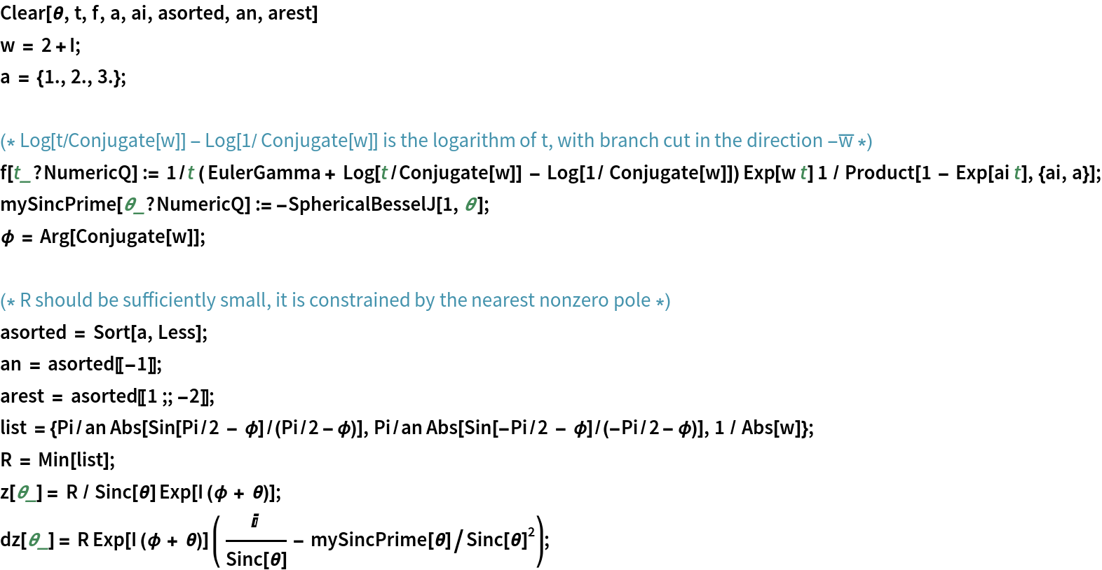 |
| In[2]:= | ![\[Theta]min = -2.7;
\[Theta]max = 2.7;
figTalbot = ParametricPlot[{Re[z[\[Theta]]], Im[z[\[Theta]]]}, {\[Theta], \[Theta]min, \[Theta]max}, PlotStyle -> Green];](https://www.wolframcloud.com/obj/resourcesystem/images/c22/c22611c4-bfa3-4e88-9dcf-1c7938329627/5769498480e031fa.png) |
| In[3]:= |  |
| In[4]:= | 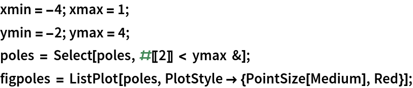 |
| In[5]:= |  |
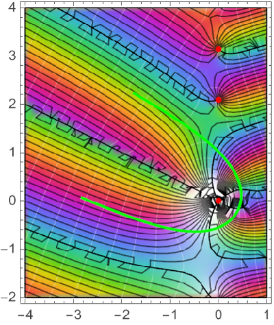
In the following figure, one sees the rotated Talbot contour (green) and selected poles of the integrand (red) in the complex t-plane. The black lines are the lines of constant phase. The colours indicate the phase of the function f. One sees that the Talbot contour more or less follows the lines of constant phase.
| In[6]:= | 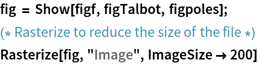 |
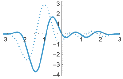
The following figure shows the integrand. Although there are oscillations, they are sufficiently mild that NIntegrate can deal with them.
| In[7]:= | ![fig2 = ReImPlot[dz[\[Theta]] f[z[\[Theta]]], {\[Theta], -3, 3}, PlotRange -> All];
(* Rasterize to reduce the size of the file *)
Rasterize[fig2, "Image", ImageSize -> 200]](https://www.wolframcloud.com/obj/resourcesystem/images/c22/c22611c4-bfa3-4e88-9dcf-1c7938329627/02a9d8f21fae7ed0.png) |
This work is licensed under a Creative Commons Attribution 4.0 International License

