Basic Examples (7)
Generate the first-order term of the Baker–Campbell–Hausdorff formula for two operators:
Generate the second-order term of the Baker–Campbell–Hausdorff formula for two operators:
Show the formula in the commutator form:
Release the commutator form and show the expanded formula:
Generate the third-order term of the Baker–Campbell–Hausdorff formula for two operators:
Show the formula in the commutator form:
Verify explicitly that the two results above are identical:
Show that the result is identical to 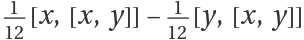 :
:
Generate the fourth-order Baker–Campbell–Hausdorff term for two operators:
Show that the result is identical to 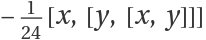 :
:
Show that the result is identical to 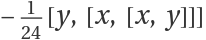 :
:
Compute the fourth-order Baker–Campbell–Hausdorff term for two operators in commutator form:
Verify explicitly that the results above are identical:
Compute the second-order Baker–Campbell–Hausdorff term for three symbolic matrices:
Compute the third-order Baker–Campbell–Hausdorff term for three operators with Composition as the action:
Compute the third-order Baker–Campbell–Hausdorff term for two operators with NonCommutativeMultiply as the action between operators:
Show the third-order Baker–Campbell–Hausdorff term for four operators with Dot as the action between operators:
Scope (2)
Show a few terms of Baker-Campbell-Hausdorff formula 𝒵=Log(ⅇX1ⅇX2…ⅇXn) with three non-commutative operators Xj:
Show the commutator form of 𝒵=Log(ⅇX1ⅇX2):
Options (2)
Show the third-order Baker–Campbell–Hausdorff term for two operators while preserving the commutator form:
Show the second-order Baker–Campbell–Hausdorff term for four symbolic matrices in commutator form:
Applications (19)
Annihilation and creation operators: (5)
The single-mode photon field satisfies the Bosonic commutation relation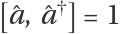 .
.
For the expression  , compute the second-order term in the Baker–Campbell–Hausdorff series:
Define a function that simplifies an noncommutative polynomial in a and a†:
Reduce (simplify) it:
Compute the third-order term of the Baker–Campbell–Hausdorff series:
Reduce it:
Likewise, the higher order terms disappear as well. Thus one finds:  .
.
Canonical position and momentum (4)
Define canonical position and momentum operators 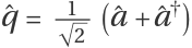 and
and 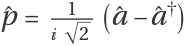 :
:
Verify 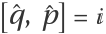 :
:
Compute the second-order term of the Baker–Campbell–Hausdorff series for 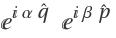 :
:
Show that the higher-order terms are zero:
Thus it means 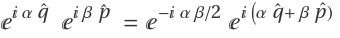 .
.
Displacement operator (3)
With the displacement operator as 𝒟(α)=ⅇα a†-α*a, show that 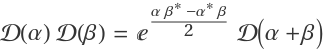 .
.
Compute the second-order term of the Baker–Campbell–Hausdorff series:
Show that the higher-order Baker–Campbell–Hausdorff terms vanish:
Compute the second through fifth terms in the BCH series of 𝒟(α1)𝒟(α2)𝒟(α3) and verify  :
:
SU(2) spin rotations (4)
Set up the variables and their SU(2) algebra[Ji,Jj]=ⅈϵijkJk with ϵ the 3-dimensional Levi-Civita totally antisymmetric tensor. Note that in our relations we do not include quadratic identities such as Jj2=𝕀, because these are representation-dependent (e.g., for Pauli matrices) rather than algebraic identities.
Given the algebra and variables, define a function to reduce a polynomial in Jj (Cartesian basis):
Consider the relation Log[ⅇ-ⅈ δt θ1J1ⅇ-ⅈ δt θ2J2]=-ⅈ δt Heff. Our goal to find effective Hamiltonian describing the above rotations. We will use rotation angles θj and also time variable δt. We should set them as scalar variable in the algebra.
Define noncommutative variables and scalars:
Compute the second-order Baker–Campbell–Hausdorff term for ⅇ-ⅈ δt θ1J1ⅇ-ⅈ δt θ2J2:
Compute Heff up to the second order of δt:
Numerical example (3)
Consider ⅇxⅇy=ⅇA with 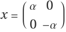 ,
, 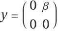 .
.
Compute the first 10 terms of the Baker–Campbell–Hausdorff series for A:
For A12 element of the matrix, show that the Taylor series of the function below matches the result above:
Therefore, one gets 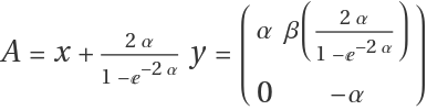
![Nest[ReleaseHold, ResourceFunction["BakerCampbellHausdorffTerms"][{x, y}, 3, "CommutatorForm" -> True], 2] - ResourceFunction["BakerCampbellHausdorffTerms"][{x, y}, 3] // NonCommutativeExpand](https://www.wolframcloud.com/obj/resourcesystem/images/557/55706fa9-2448-430a-aeaa-b510e5f5c081/2b897bc2e2c983ee.png)
![ResourceFunction["BakerCampbellHausdorffTerms"][{x, y}, 3] - 1/12 (Commutator[x, Commutator[x, y]] - Commutator[y, Commutator[x, y]]) // NonCommutativeExpand](https://www.wolframcloud.com/obj/resourcesystem/images/557/55706fa9-2448-430a-aeaa-b510e5f5c081/2c5e4e5d0e951abf.png)
![ResourceFunction["BakerCampbellHausdorffTerms"][{x, y}, 4] - (-(1/24) Commutator[x, Commutator[y, Commutator[x, y]]]) // NonCommutativeExpand](https://www.wolframcloud.com/obj/resourcesystem/images/557/55706fa9-2448-430a-aeaa-b510e5f5c081/1049a5002a01ae19.png)
![ResourceFunction["BakerCampbellHausdorffTerms"][{x, y}, 4] - (-(1/24) Commutator[y, Commutator[x, Commutator[x, y]]]) // NonCommutativeExpand](https://www.wolframcloud.com/obj/resourcesystem/images/557/55706fa9-2448-430a-aeaa-b510e5f5c081/43a0afb2648675bd.png)
![Nest[ReleaseHold, ResourceFunction["BakerCampbellHausdorffTerms"][{x, y}, 4, "CommutatorForm" -> True], 3] - ResourceFunction["BakerCampbellHausdorffTerms"][{x, y}, 4] // NonCommutativeExpand](https://www.wolframcloud.com/obj/resourcesystem/images/557/55706fa9-2448-430a-aeaa-b510e5f5c081/249ab7a9cbac97e2.png)


![With[{ops = Table[ToString[Subscript[x, j], StandardForm], {j, 3}]},
Grid[Table[{ToString[Subscript[\[ScriptCapitalZ], j], StandardForm], ResourceFunction["BakerCampbellHausdorffTerms"][ops, j, Dot] // NonCommutativeExpand[#, Dot] &}, {j, 4}], Frame -> All, Alignment -> Left]]](https://www.wolframcloud.com/obj/resourcesystem/images/557/55706fa9-2448-430a-aeaa-b510e5f5c081/79cce210aa59a47d.png)

![Grid[Table[{ToString[Subscript[\[ScriptCapitalZ], j], StandardForm], ResourceFunction["BakerCampbellHausdorffTerms"][{x, y}, j, "CommutatorForm" -> True] // TraditionalForm}, {j, 5}], Frame -> All, Alignment -> Left]](https://www.wolframcloud.com/obj/resourcesystem/images/557/55706fa9-2448-430a-aeaa-b510e5f5c081/2a6f7503263b646e.png)

![ClearAll[NCPolynomialReductionBosonic]
NCPolynomialReductionBosonic[exp_, scalars_ : {}] := NonCommutativePolynomialReduce[
exp, {Commutator[a, SuperDagger[a]] - 1}, {a, SuperDagger[a]}, NonCommutativeAlgebra[<|"ScalarVariables" -> scalars|>]][[-1]]](https://www.wolframcloud.com/obj/resourcesystem/images/557/55706fa9-2448-430a-aeaa-b510e5f5c081/4ee95bdf21c6b49a.png)


![Table[NCPolynomialReductionBosonic[
ResourceFunction[
"BakerCampbellHausdorffTerms"][{I \[Alpha] q, I \[Beta] p}, n], {\[Alpha], \[Beta]}], {n, 3, 6}]](https://www.wolframcloud.com/obj/resourcesystem/images/557/55706fa9-2448-430a-aeaa-b510e5f5c081/78dd7924aa8a7e1e.png)

![NCPolynomialReductionBosonic[
ResourceFunction[
"BakerCampbellHausdorffTerms"][{\[Alpha] SuperDagger[a] - Conjugate[\[Alpha]] a, \[Beta] SuperDagger[a] - Conjugate[\[Beta]] a}, 2], {\[Alpha], \[Beta]}]](https://www.wolframcloud.com/obj/resourcesystem/images/557/55706fa9-2448-430a-aeaa-b510e5f5c081/7cfba27aa79e6d7c.png)
![Table[NCPolynomialReductionBosonic[
ResourceFunction[
"BakerCampbellHausdorffTerms"][{\[Alpha] SuperDagger[a] - Conjugate[\[Alpha]] a, \[Beta] SuperDagger[a] - Conjugate[\[Beta]] a}, n], {\[Alpha], \[Beta]}], {n, 3, 6}]](https://www.wolframcloud.com/obj/resourcesystem/images/557/55706fa9-2448-430a-aeaa-b510e5f5c081/078e4c8d2bd57dd5.png)
![Table[NCPolynomialReductionBosonic[
ResourceFunction["BakerCampbellHausdorffTerms"][
Table[Subscript[\[Alpha], j] SuperDagger[a] - Conjugate[Subscript[\[Alpha], j]] a, {j, 3}], n], Table[Subscript[\[Alpha], j] , {j, 3}]], {n, 2, 5}]](https://www.wolframcloud.com/obj/resourcesystem/images/557/55706fa9-2448-430a-aeaa-b510e5f5c081/6799165469ad9710.png)

![ClearAll[NCPolynomialReductionSU2]
NCPolynomialReductionSU2[exp_, vars_, scalars_ : {}, scale_ : 1] /; Length[vars] == 3 := NonCommutativePolynomialReduce[exp, DeleteCases[0]@
Flatten@(Outer[Commutator, vars, vars] - I scale TensorContract[
TensorProduct[LeviCivitaTensor[3], vars], {{3, 4}}]), {vars},
NonCommutativeAlgebra[<|"ScalarVariables" -> scalars|>]][[-1]]](https://www.wolframcloud.com/obj/resourcesystem/images/557/55706fa9-2448-430a-aeaa-b510e5f5c081/030bc3215efc51c1.png)
![Sum[NCPolynomialReductionSU2[
ResourceFunction[
"BakerCampbellHausdorffTerms"][{-I \[Delta]t Subscript[\[Theta], 1] Subscript[J, 1], -I \[Delta]t Subscript[\[Theta], 2]
Subscript[J, 2]}, n], vars, scalars], {n, 3}]/(-I \[Delta]t) // Expand](https://www.wolframcloud.com/obj/resourcesystem/images/557/55706fa9-2448-430a-aeaa-b510e5f5c081/74e8617395dd575a.png)
![x = \[Alpha] PauliMatrix[3]; y = {{0, \[Beta]}, {0, 0}};
A = Sum[ResourceFunction["BakerCampbellHausdorffTerms"][{x, y}, n, Dot], {n, 11}];
A // MatrixForm](https://www.wolframcloud.com/obj/resourcesystem/images/557/55706fa9-2448-430a-aeaa-b510e5f5c081/742b94cfd660bd71.png)
![Normal[\[Beta] Series[(2 \[Alpha])/(
1 - Exp[-2 \[Alpha]]), {\[Alpha], 0, 10}]] == A[[1, 2]]](https://www.wolframcloud.com/obj/resourcesystem/images/557/55706fa9-2448-430a-aeaa-b510e5f5c081/7733570bb909cb76.png)