Function Repository Resource:

ApproximatePolynomialGCD

Compute an approximate GCD to a pair of polynomials with approximate coefficients

Contributed by: Daniel Lichtblau

ResourceFunction["ApproximatePolynomialGCD"][poly₁,poly₂]

computes a polynomial that is, to reasonable approximation, a largest-degree divisor of both poly₁ and poly₂.

Details and Options

ResourceFunction["ApproximatePolynomialGCD"] takes a Tolerance option with default of 10^-5.

ResourceFunction["ApproximatePolynomialGCD"] uses numeric substitutions with complex values. This can lead to results where all input coefficients are real-valued and yet imaginary parts appear. In such cases these imaginary parts are removed.

The tolerance is used primarily to remove terms that are too small to be considered relevant.

ResourceFunction["ApproximatePolynomialGCD"] handles the univariate case using singular value decompositions on Sylvester matrices. A secondary use of the Tolerance option is to determine which singular values to regard as zero.

The multivariate case is handled by iteratively solving linear overdetermined least-squares systems to compute cofactors and partial greatest common divisors, lifting one variable at a time.

Examples are from user questions in forums and benchmarks from the literature on approximate polynomial GCDs.

Examples

Basic Examples (2)

Compute the approximate GCD of a pair of univariate polynomials:

In[1]:=

p1 = x^14 + 3.00001 x^10 - 7.99998 x^7 - 25.00002 x^6 + 3.00001 x^13 + 9.00006 x^9 - 3.00001 x^5 - 2.00001 x^8 - 6.00005 x^4 + 16.00004 x + 2.00001;
p2 = x^13 - 3.00003 x^9 - 2.99999 x^6 + 2.99999 x^12 - 9.00006 x^8 - 8.99997 x^5 - 1.99998 x^7 + 5.99999 x^3 + 5.99994;
approxgcd = ResourceFunction["ApproximatePolynomialGCD"][p1, p2]

Out[3]=

Compare to the GCD from rounding the coefficients of these polynomials:

In[4]:=

Out[5]=

They are very close up to a constant multiple:

In[6]:=

Out[6]=

Compute the approximate GCD of a pair of bivariate polynomials:

In[7]:=

${f, g} = {x^3 - 8.05690292794*x^2*y + 66.8206602296*x^2 - 2.42037371481*x*y^2 + 17.8341472094*x*y - 55.3041827489*x + 8.52288118623*y^3 - 66.7864893146*y^2 - 35.9578468971*y + 71.4328040275, -1.7128257326*x^2*y - 0.309381807141*x^2 + 13.9547615636*x*y^2 - 111.58197742*x*y - 20.6540588108*x + 1.0984988335*y^3 - 23.4487086797*y^2 + 116.275997087*y + 18.7247500823}; ResourceFunction["ApproximatePolynomialGCD"][f, g]$

Out[8]=

Scope (2)

Perturb a factor to create a pair of bivariate polynomials with an approximate factor in common:

In[9]:=

$ggg = -84 + 41 x + 23 y + 99 x^2 y^5 - 61 x^2 y^4 - 50 x^2 y^3 - 12 x^2 y^2 - 18 x^2 y - 26 x y^7 - 62 x y^6 + x y^5 - 47 x y^4 - 91 x y^3 - 47 x y^2 + 66 x^3 y - 55 x^7 y - 35 x^6 y^2 + 97 x^6 y + 79 x^5 y^3 + 56 x^5 y^2 + 49 x^5 y + 57 x^4 y^4 - 59 x^4 y^3 + 45 x^4 y^2 - 8 x^4 y + 92 x^3 y^5 + 77 x^3 y^2 + 54 x^3 + 53 y^6 + 31 x^2 - 90 y^7 - 58 y^8 - 85 x^8 - 37 x^7 - 86 y^2 + 50 x^6 + 83 y^3 + 63 x^5 + 94 y^4 - 93 x^4 - y^5 - 5 x^2 y^6 - 61 x y + 43 x^3 y^4 - 62 x^3 y^3; hhh = -76 - 53 x + 88 y + 66 x^2 y^5 - 29 x^2 y^4 - 91 x^2 y^3 - 53 x^2 y^2 - 19 x^2 y + 68 x y^6 - 72 x y^5 - 87 x y^4 + 79 x y^3 + 43 x y^2 + 80 x^3 y - 50 x^6 y - 53 x^5 y^2 + 85 x^5 y + 78 x^4 y^3 + 17 x^4 y^2 + 72 x^4 y + 30 x^3 y^2 + 72 x^3 - 23 y^6 - 47 x^2 - 61 y^7 + 19 x^7 - 42 y^2 + 88 x^6 - 34 y^3 + 49 x^5 + 31 y^4 - 99 x^4 - 37 y^5 - 66 x y - 85 x^3 y^4 - 86 x^3 y^3; poly1 = Expand[ggg*hhh]; randomPoly[deg_, vars_] := Module[{n = Length[vars], t, poly, terms}, poly = RandomInteger[{-10, 10}, {deg + 1}] . t^Range[0, deg]; Expand[ poly /. t^j_. :> (RandomInteger[{-5, 5}, {Length[vars]}] . vars)^j]] SeedRandom[1111]; mmm = randomPoly[7, {x, y}]; poly2 = Expand[(ggg + 1/1000 - 3/1000*x + 7/1000*y)* mmm];$

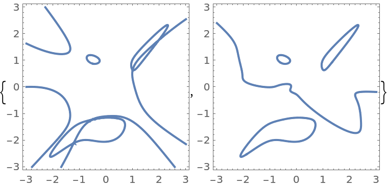
Some of zero contours are quite similar:

In[10]:=

Out[10]=

Recover the approximate GCD:

In[11]:=

Out[11]=

Check that the result, suitably normalized, is close to the known approximate common factor:

In[12]:=

$Chop[Expand[approxgcd*(ggg/approxgcd /. {x -> 0, y -> 0})] - ggg, 5*10^(-3)]$

Out[12]=

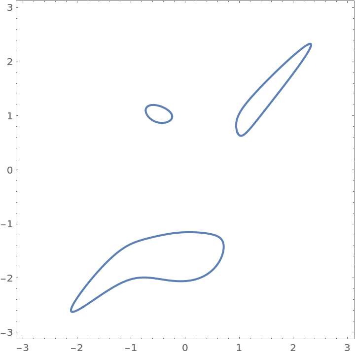
The zero contour of the approximate GCD is similar to the similar contours from the inputs:

In[13]:=

Out[13]=

A large trivariate example:

In[14]:=

(* Evaluate this cell to get the example input *) CloudGet["https://www.wolframcloud.com/obj/0682bfff-1621-493e-8da1-9c71f4f152f4"]

Compute the approximate GCD:

In[15]:=

Out[15]=

Find the GCD of the unnoised polynomials:

In[16]:=

Out[16]=

Normalize and check that the difference is close to zero:

In[17]:=

$Chop[Expand[ gcd*(approxgcd/gcd /. {x -> 0, y -> 0, z -> 0}) - approxgcd], 10^(-5)]$

Out[17]=

Possible Issues (3)

Create a system with a known GCD and add a large noise term in y² to the second polynomial along with several smaller noise terms:

In[18]:=

p = 3 + y + 5 x + w + 2 x^2;
f = p*(3 + 4 y + 3 x) + .04*y + .03*x + .01*x*y + .04*y^3;
g = p*(2 + y + 5 x) + .06 + .02*x*y + .006 y^2 + .04*x^3; g6 = g + 6 y^2;

A large tolerance can allow an approximate GCD to have terms of excessive degree:

In[19]:=

Out[19]=

With a tighter tolerance these disappear:

In[20]:=

Out[20]=

Requirements

Wolfram Language 13.0 (December 2021) or above

Version History

1.0.0 – 08 July 2024

Source Metadata

Citation:
- Robert Corless, Patrizia Gianni, Barry Trager and Stephen Watt. The singular value decomposition for polynomial systems. Proceedings of the 1995 International Symposium on Symbolic and Algebraic Computation (ISSAC 95), 195207, 1995. ACM Press. DOI: 10.1145/220346.220371
- Robert Corless, Mark Giesbrecht, Mark van Hoeij, Ilias Kotsireas and Stephen Watt. Towards factoring bivariate approximate polynomials. Proceedings of the 2001 International Symposium on Symbolic and Algebraic Computation (ISSAC 2001), 8592, 2001. ACM Press. DOI: 10.1145/384101.38411
- Erich Kaltofen, Zhengfeng Yang and Lihong Zhi. Proceedings of the 2006 International Symposium on Symbolic and Algebraic Computation (ISSAC 06), 169176, 2006. ACM Press. DOI: 10.1145/1145768.1145799
  Examples available from: Erich Kaltofen's Homepage
- Masaru Sanuki. Computing approximate GCD of multivariate polynomials. Proceedings of the 2005 International Workshop on Symbolic-numeric Computation (SNC 05), 5568, 2005. Trends in Mathematics, Birkhäuser.
- Daniel Lichtblau. Approximate polynomial GCD by approximate syzygies. Mathematics in Computer Science 13:517-523, 2119. DOI: 10.1007/s11786-019-00392-w

Related Resources

Author Notes

While several citations are provided, these are mostly for the examples and to give some idea of methods that have been introduced. The code here is, in one form or another, what is commonly used for the univariate case. The lifting strategy appears to be new. While it seems to work well on a variety of benchmarks, it certainly has limitations. It is expected that large examples (high degree and/or many variables) will run out of memory in the linear algebra steps or else give results that are far from expected (in those cases where an approximate GCD is in the actual construction). Some code is in place to lessen this likelihood by using a suitable multiplier matrix to keep the number of rows not much larger than the number of columns in the least-squares steps. This however has the unfortunate effect of decreasing the quality of the results, so it is only put to use when dimensions exceed a threshold.

The lifting method could likely be made to use less memory by iterative corrections one degree at a time, as in linear Hensel lifting. This approach might be considered for a future update.

An exact variant of this method, using suitable complex values of modulus 1, could also be considered. Similarly one might try to handle the case of computing over a finite field, again using suitable numeric substitutions. It is not clear whether such an approach could be made competitive with existing methods for those cases.

License Information

This work is licensed under a Creative Commons Attribution 4.0 International License

Wolfram Function Repository

ApproximatePolynomialGCD

Details and Options