Function Repository Resource:

AlgebraicRange

Source Notebook

Generate ranges of algebraic numbers

Contributed by: Daniele Gregori

ResourceFunction["AlgebraicRange"][x]

gives the range of square roots Sqrt[Range[1,x^2]], for x>=1.

ResourceFunction["AlgebraicRange"][x,y]

gives the range of square roots Sqrt[Range[x^2,y^2]], for 0<=x<=y.

ResourceFunction["AlgebraicRange"][x,y,s]

generates steps bounded above by s, with 0<s<=y.

ResourceFunction["AlgebraicRange"][x,y,s,d]

requires the steps to be bounded below by d, with 0<=d<=s.

Details and Options

AlgebraicRange creates ranges made of algebraic numbers. This extends the basic concept of Range to include, besides Rational numbers, also roots, always restricted to the Reals domain.

The first two arguments represent the bounds of the range (minimum and maximum values), while the optional third and fourth arguments (by default equal to 1 and 0) regulate the upper and lower bounds of the steps (differences between successive elements).

If no step parameter is specified, the elementary algebraic range ResourceFunction["AlgebraicRange"][x,y] is determined by the square root range Sqrt[Range[x^2,y^2]], for x,y>0. The extension to negative bounds x <0 or y<0 is performed simply by reflection, since general real roots are mathematically defined only for positive arguments.

The step between successive algebraics is not straightforward to define univocally, as there exists no constant difference among the irrational numbers generated even with the elementary algebraic range. However, it turns out that an intuitively simple class of algebraic ranges, with non-unit step parameter s, is obtained by taking the Outer product of ResourceFunction["AlgebraicRange"][Min[x,x/s],y] with Join[Range[0,Max[1, s], s], Range[Max[1, s], y, s]], for 0<s<=y-x and 0<=x<=y. Then the parameter s also becomes the upper bound for all the steps. For example,

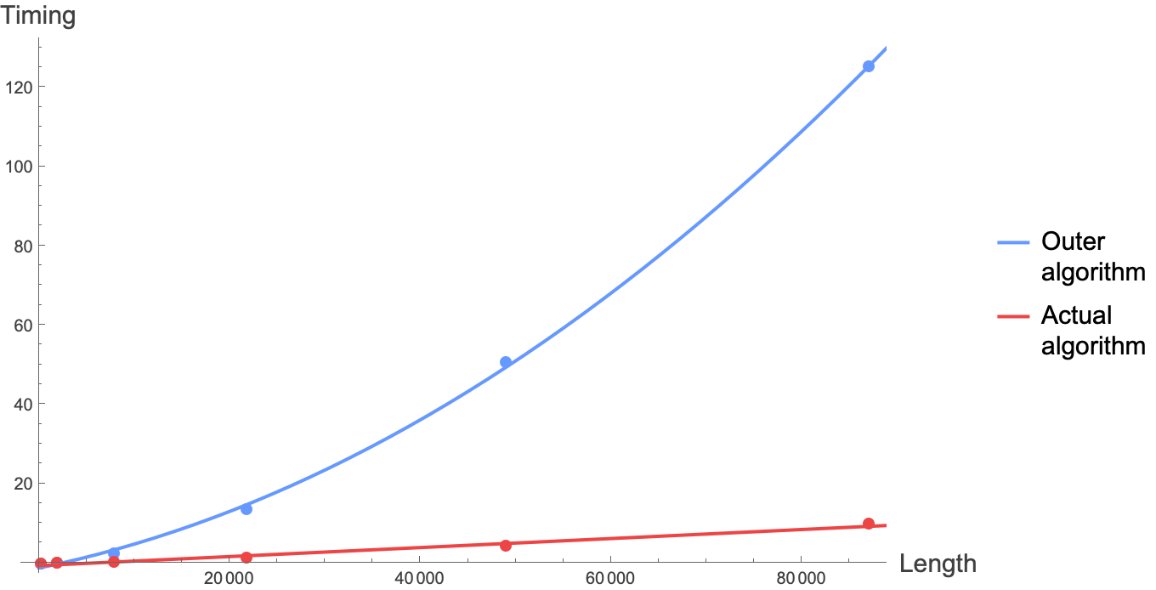
This definition of algebraic step is more easily conveyed in terms of Outer, but if implemented literally it would lead to an intrinsically inefficient algorithm, for which Timing would scale quadratically with respect to the size of the input arguments. Thus, the actual algorithm implemented by ResourceFunction["AlgebraicRange"] generates output equivalent to Outer but is internally more refined - crucially leveraging the function Nearest inside For loops - and effectively scales with linear time complexity.

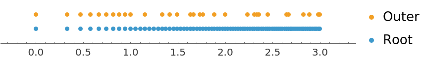
The algebraic numbers thus generated can often be in a great number, with a tendency to accumulate towards certain points. To avoid these features, a further fourth argument d can be optionally provided to require a minimum (absolute value) difference between successive algebraics, that is a lower bound for all the steps. This truncation process typically leads to a nearly uniform distribution of numeric values.

Extended functionality and syntax, especially for creating algebraic numbers of a more general form, are provided in the homonymous function of the paclet DanieleGregori/GeneralizedRange.

A natural application of AlgebraicRange is in the search for closed forms for floating point numbers, possibly in terms of arbitrary combinations of mathematical functions with algebraic arguments, through ResourceFunction["FindClosedForm"].

ResourceFunction["AlgebraicRange"] accepts the following options:

"RootOrder"

the root orders to be included

"StepMethod"

"Outer"

change the method to define the step

"FareyRange"

False

generate algebraic numbers with steps given by the Farey sequence

"FormulaComplexity"

Infinity

set a complexity threshold over which the algebraics are discarded

"AlgebraicsOnly"

True

accept only algebraic arguments and output

WorkingPrecision

MachinePrecision

set the precision for all internal numerical evaluations

The option "RootOrder" can take the following values:

include roots up to r order

{r}

include only roots of order r

{r₁,r₂,…}

include roots of all specified orders r_k

The option "StepMethod" can be used to define the step in ResourceFunction["AlgebraicRange"][x,y,s] and can take the following values, for 0<=x<=y, 0<s<=y-x:

"Outer"

take the Outer product of ResourceFunction["AlgebraicRange"][Min[x,x/s],y] with Join[Range[0,Max[1, s], s]],Range[Max[1, s], y, s]]

"Root"

use Sqrt[Range[x^2,y^2,s^2]]

A more detailed explanation of the step definition, also for negative arguments, can be found in the Properties and Relations examples.

Besides using the fourth argument to impose a lower bound on the steps, another way to restrict the output of ResourceFunction["AlgebraicRange"] is by setting a threshold for the complexity of the numeric expressions involved through the option "FormulaComplexity". The corresponding numerical values are not meaningful in practice and should be determined through a heuristic approach. A user interested in precise computations of the underlying homonymous function may use the paclet "DanieleGregori/GeneralizedRange".

Examples

Basic Examples (2)

Generate a range of square roots:

In[1]:=

Out[1]=

In[2]:=

Out[2]=

Generate a square root range with non-unit step:

In[3]:=

Out[3]=

In[4]:=

Out[4]=

Scope (4)

Generate a range of negative square roots:

In[5]:=

Out[5]=

In[6]:=

Out[6]=

Generate a range of mixed positive and negative roots, with a negative step:

In[7]:=

Out[7]=

In[8]:=

Out[8]=

Generate a range of square roots, with certain upper and lower bounds on the steps:

In[9]:=

Out[9]=

In[10]:=

Out[10]=

In[11]:=

Out[11]=

Generate a range of nested square roots:

In[12]:=

Out[12]=

Options (15)

RootOrder (4)

Generate a range of square and cubic roots:

In[13]:=

Out[13]=

Generate a range of fourth roots:

In[14]:=

Out[14]=

Generate a range of cube and fifth roots:

In[15]:=

Out[15]=

Generate algebraic terms up to fourth root order and require a minimum absolute difference between successive roots:

In[16]:=

Out[16]=

StepMethod (2)

Change method to define the step:

In[17]:=

Out[17]=

Compare with the default "Outer" step method:

In[18]:=

Out[18]=

In[19]:=

Out[19]=

FareyRange (2)

Generate an algebraic range that generalizes ResourceFunction["FareyRange"]:

In[20]:=

Out[20]=

In[21]:=

Out[21]=

In[22]:=

Out[22]=

Notice that the step parameter is originally the denominator of the step (both it and its reciprocal are accepted). This corresponds to the Union of ranges with steps equal to the elements of the FareySequence:

In[23]:=

Out[23]=

In[24]:=

Out[24]=

FormulaComplexity (3)

With the default option "FormulaComplexity" set to Infinity, a very large number of algebraics can be produced:

In[25]:=

Out[25]=

In[26]:=

Out[26]=

One way to limit these is by using the fourth argument, to require a minimum absolute difference between successive algebraics:

In[27]:=

Out[27]=

In[28]:=

Out[28]=

An alternative way is by setting the option "FormulaComplexity" to a finite threshold value, to select only numeric symbols with complexity less than that:

In[29]:=

Out[29]=

In[30]:=

Out[30]=

WorkingPrecision (2)

If the step parameter is too small, some algebraic numbers may collide in their numerical values and get omitted in the output:

In[31]:=

$machPrecRg = With[{s = 10^(-17)}, ResourceFunction["AlgebraicRange"][Sqrt[1 - 25 s], Sqrt[1 + 25 s], s]]$

Out[31]=

In[32]:=

Out[32]=

To avoid this, increase the value of the option WorkingPrecision:

In[33]:=

$highPrecRg = With[{s = 10^(-17)}, ResourceFunction["AlgebraicRange"][Sqrt[1 - 25 s], Sqrt[1 + 25 s], s, WorkingPrecision -> 20]];$

In[34]:=

Out[34]=

In[35]:=

Out[35]=

Precision can be pushed arbitrarily high:

In[36]:=

$highPrecRg2 = Block[{s = 10^(-50), $MaxExtraPrecision = 100}, ResourceFunction["AlgebraicRange"][Sqrt[1 - 2 s], Sqrt[1 + 2 s], s, WorkingPrecision -> 60]]$

Out[36]=

In[37]:=

Out[37]=

AlgebraicsOnly (2)

By default, only algebraic numbers are accepted as input parameters:

In[38]:=

Out[38]=

Set this option to deliberately accept an output range which includes transcendental numbers:

In[39]:=

Out[39]=

In[40]:=

Out[40]=

Applications (2)

AlgebraicRange[x,y] is naturally suited for searching possible closed forms through ResourceFunction["FindClosedForm"]:

In[41]:=

Out[41]=

In[42]:=

Out[42]=

Compare with the more complex result found with the "Plain" rational range:

In[43]:=

Out[43]=

In[44]:=

Out[44]=

AlgebraicRange[x,y,s] provides a more general search range:

In[45]:=

Out[45]=

In[46]:=

Out[46]=

The built-in function RootApproximant may have difficulty recognizing even relatively simple nested roots:

In[47]:=

Out[47]=

In[48]:=

Out[48]=

In principle, these may be recognized by equipping ResourceFunction["FindClosedForm"] with a suitable search range in terms of AlgebraicRange[x,y,s]:

In[49]:=

ResourceFunction["FindClosedForm"][10.13051909, Identity, "SearchRange" -> Function[
Join[ResourceFunction["AlgebraicRange"][1, #, 1/2], ResourceFunction["AlgebraicRange"][Sqrt[1 + Sqrt[2]], #, 1/Sqrt[2]]]]]

Out[49]=

Properties and Relations (7)

AlgebraicRange[x,y] always extends Range[x,y] if x, y are integers:

In[50]:=

Out[50]=

In[51]:=

Out[51]=

In[52]:=

Out[52]=

The extension may not be complete for rational or irrational arguments:

In[53]:=

Out[53]=

In[54]:=

Out[54]=

In[55]:=

Out[55]=

AlgebraicRange[x,y] for x<=y<0 is equivalent to Reverse[-AlgebraicRange[-y,-x]]:

In[56]:=

Out[56]=

In[57]:=

Out[57]=

Compute the algebraic range for 0<=x<=y and positive step upper bound s>0:

In[58]:=

Out[58]=

This is an equivalent calculation:

In[59]:=

Out[59]=

An algebraic range with a negative irrational step size:

In[60]:=

Out[60]=

An equivalent calculation:

In[61]:=

Select[ReverseSortBy[
Outer[Times, Join[Range[0, 1, 1/Sqrt[3]], Range[1, 3, 1/Sqrt[3]]], Range[3^2, (3/2)^2, -1]^(1/2)] // Flatten // DeleteDuplicates, N],
3/2 <= # <= 3 &]

Out[61]=

The starting point is always preserved:

In[62]:=

Out[62]=

In[63]:=

Out[63]=

In[64]:=

Out[64]=

In[65]:=

Out[65]=

The numbers generated always belong to the domains of Algebraics and Reals:

In[66]:=

algrange = Block[{$MaxExtraPrecision = 200000}, ResourceFunction["AlgebraicRange"][
2 Sqrt[1 + Sqrt@RandomInteger[{2, 5}]], -2 Sqrt[
1 + Sqrt@RandomInteger[{2, 5}]], -Sqrt[2]/RandomInteger[{2, 5}], 1/4, "RootOrder" -> RandomInteger[{2, 5}, 2]]]

Out[66]=

In[67]:=

Out[67]=

In[68]:=

Out[68]=

Possible Issues (3)

Only real arguments are accepted:

In[69]:=

Out[69]=

A simple numeric input can be automatically recognized with its exact expression:

In[70]:=

Out[70]=

In[71]:=

Out[71]=

However, some numeric input is not adequately recognized:

In[72]:=

Out[72]=

In[73]:=

Out[73]=

In any case, the numeric difference with the corresponding exact expressions remains negligible:

In[74]:=

Out[74]=

In[75]:=

Out[75]=

In[76]:=

Out[76]=

Introducing a lower bound may cause the upper bound not to be respected anymore:

In[77]:=

Out[77]=

In[78]:=

Out[78]=

Neat Examples (2)

The implementation of AlgebraicRange[x,y,s] for step parameter s!=1 is more easily conveyed in terms of Outer as follows:

In[79]:=

outerAlgebraicRange[x_, y_, s_] /; x <= y && 0 < s <= y - x :=
Select[
SortBy[
Outer[
Times,
Join[
Range[0, Max[1, s], s],
Range[Max[1, s], Max[Abs[x], Abs[y]], s]],
ResourceFunction["AlgebraicRange"][
If[x > 0, Min[x, x/s], Max[x, x/s]],
y]]
// Flatten,
N],
x <= # <= y &] //
DeleteDuplicatesBy[N]

In[80]:=

Out[80]=

In[81]:=

Out[81]=

In[82]:=

Out[82]=

This apparently complicated definition has the advantage of typically leading to an output with shorter Length and which is less complex, say, in terms of LeafCount, than merely applying Sqrt to the Range of squared arguments:

In[83]:=

In[84]:=

Out[84]=

In[85]:=

Out[85]=

In[86]:=

Out[86]=

However, the above implementation in terms of Outer is also essentially inefficient, as it scales with quadratic time complexity with respect to the size of the input bounds or the length of the output range. The actual implementation of AlgebraicRange[x,y,s] is equivalent in terms of output result but it is also much more efficient, scaling with nearly linear time complexity.

Let us directly compare the performance of the outer and actual algorithms by an explicit computation, conveniently delegated to RemoteBatchSubmit:

In[87]:=

In[88]:=

job = RemoteBatchSubmit[ CompoundExpression[ timesO = {}; timesA = {}; lens = {}; checks = {};, Table[ Block[{resO, resA, timeO, timeA, check, len}, {timeO, resO} = outerAlgebraicRange[0, r, 1/2] // RepeatedTiming;
AppendTo[timesO, timeO]; {timeA, resA} = ResourceFunction["AlgebraicRange"][0, r, 1/2] // RepeatedTiming;
AppendTo[timesA, timeA]; check = resO == resA;
AppendTo[checks, check]; len = Length[resA];
AppendTo[lens, len];], {r, maxs}], <|"Bound" -> maxs, "Match" -> checks, "Length" -> lens, "Time Outer" -> timesO, "Time Actual" -> timesA|>], RemoteMachineClass -> "Basic4x16"]

Out[88]=

After a few minutes (and a few credits spent) we get back the result:

In[89]:=

Out[89]=

In[90]:=

Out[90]=

In[91]:=

Out[91]=

In[92]:=

Out[92]=

Also in Tabular form:

In[93]:=

Out[93]=

Let us plot the resulting RepeatedTiming against the output Length, together with their quadratic and linear fits:

In[94]:=

$With[ {AC = ResourceFunction["AssociateColumns"]}, {lsLenTO = List @@@ Normal@AC[tabResults, "Length" -> "Time Outer"], lsLenTA = List @@@ Normal@AC[tabResults, "Length" -> "Time Actual"]}, {quadfit = NonlinearModelFit[lsLenTO, a x^2 + b x + c, {a, b, c}, x] // Normal, linfit = LinearModelFit[lsLenTA, x, x] // Normal, colors = {StandardBlue, StandardRed}, pt = 15, lsMax = Max[tabResults[All, "Length"] // Normal]}, Show[ ListPlot[ {lsLenTO, lsLenTA}, PlotStyle -> Evaluate[Directive[#, PointSize[Large]] & /@ colors], PlotRange -> All], Plot[{quadfit, linfit}, {x, 0, 10^Ceiling[Log10[lsMax]]}, PlotLegends -> {Style["Outer\nalgorithm", pt], Style["Actual\nalgorithm", pt]}, PlotStyle -> colors], AxesLabel -> {Style["Length", pt], Style["Timing", pt]}, ImageSize -> Large]]$

Out[94]=

Publisher

Daniele Gregori

Requirements

Wolfram Language 13.0 (December 2021) or above

Version History

2.0.0 – 08 April 2026
1.0.0 – 29 October 2025

Related Resources

Author Notes

Extended functionality is provided in the homonymous function of the paclet "DanieleGregori/GeneralizedRange".

Change Log

Version 2.0.0

More natural definition for negative bounds and non-unit step parameters, in some cases not backward compatible.

Improved algorithm for non-unit step parameter (under the default option "StepMethod" → "Outer"), now scaling with linear time complexity.

Implementation of the new option WorkingPrecision, allowing generation of arbitrarily fine ranges.

Various other code and efficiency improvements.

Verified comprehensive tests and benchmarks.

License Information

This work is licensed under a Creative Commons Attribution 4.0 International License

Wolfram Function Repository

AlgebraicRange

Details and Options

Examples

Basic Examples (2)

Scope (4)

Options (15)

RootOrder (4)

StepMethod (2)

FareyRange (2)

FormulaComplexity (3)

WorkingPrecision (2)

AlgebraicsOnly (2)

Applications (2)

Properties and Relations (7)

Possible Issues (3)

Neat Examples (2)

Publisher

Related Links

Requirements

Version History

Related Resources

Author Notes

Change Log

Version 2.0.0

License Information

AlgebraicRange

Details and Options

Examples

Basic Examples (2)

Scope (4)

Options (15)

RootOrder (4)

StepMethod (2)

FareyRange (2)

FormulaComplexity (3)

WorkingPrecision (2)

AlgebraicsOnly (2)

Applications (2)

Properties and Relations (7)

Possible Issues (3)

Neat Examples (2)

Publisher

Related Links

Requirements

Version History

Related Resources

Related Symbols

Author Notes

Change Log

Version 2.0.0

License Information