Basic Examples (10)
Find symbolic roots of fractional derivatives of polynomials with exact coefficients:
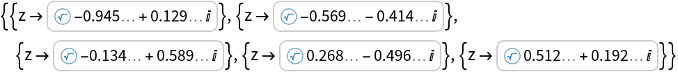
Show the explicit Root objects:
Find numeric roots of fractional derivatives of polynomials with inexact coefficients:
Use a higher working precision to get arbitrary-precision results:
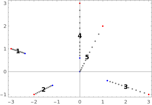
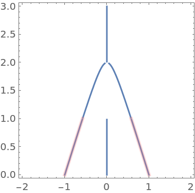
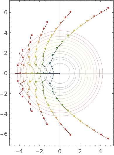
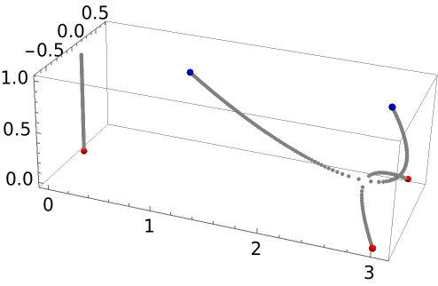
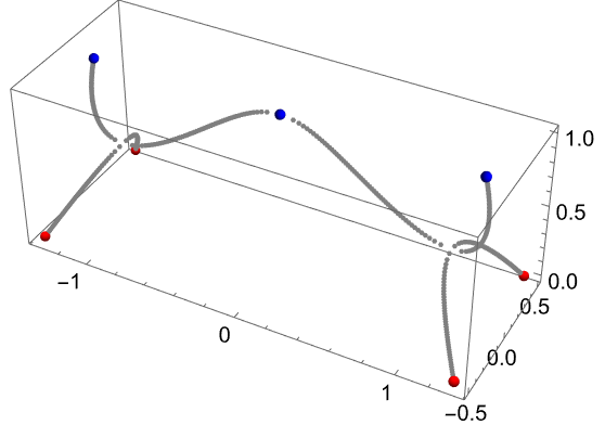
Visualize the movement of the roots of a quintic polynomial when the polynomial is differentiated:
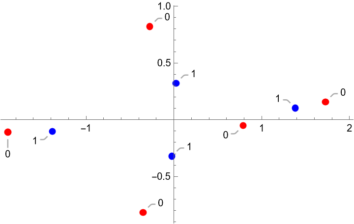
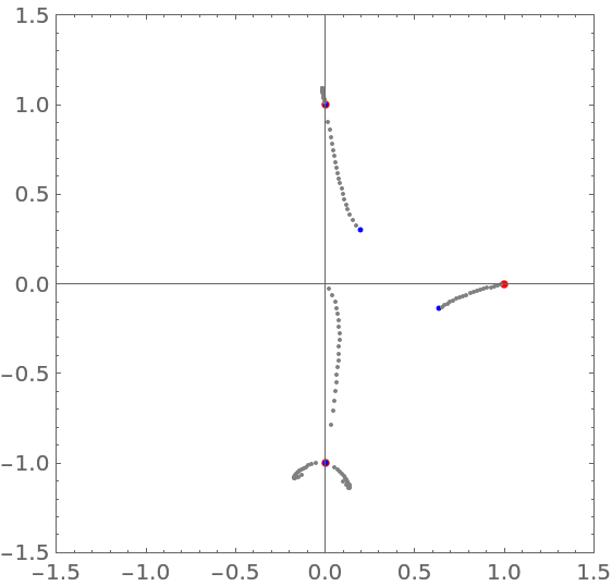
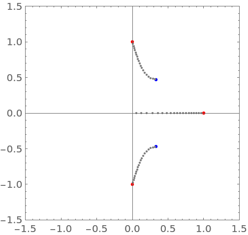
Plot the roots of the polynomial in red and the roots of the derivative of the polynomial in blue:
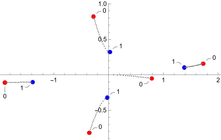
Add the roots of the fractional derivative of order α for some α from the interval (0,1) (three of the four roots of the polynomial smoothly become the three roots of the differentiated polynomial, and one root moves to the origin):
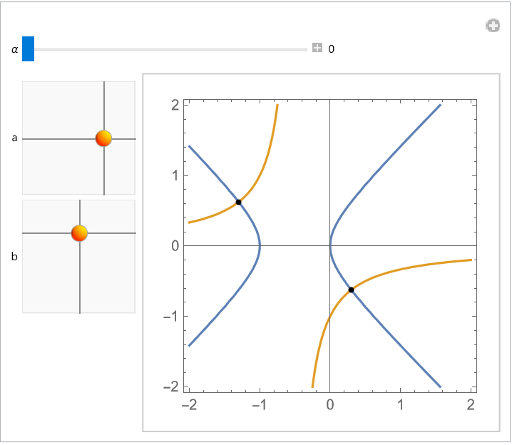
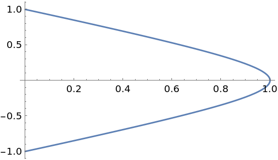
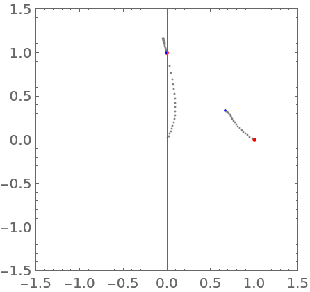
Find the defining equation for the roots of fractional order of a generic quadratic equation:
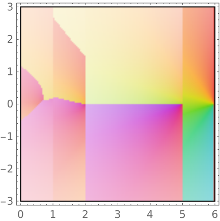
Visualize the roots of this equation for 0≤α<1 as the intersection of vanishing real and imaginary parts:
Equation for the roots of fractional order of a generic cubic equation:
The factorial expressions containing α can be reduced to rational functions in α through the identity (n-α)!⧴(-α)!∏k=1n(k-α):
Use the identity to obtain a form of the equation for 0≤α<1:
The equation for the roots becomes a polynomial with coefficients that are polynomial in α:
For α≈0, the leading term becomes the original polynomial, and one factor of the leading term for α≈1 is the differentiated polynomial:
Equation for the roots of fractional order of a generic cubic equation:
Equation for the roots of fractional order of a generic quartic equation:
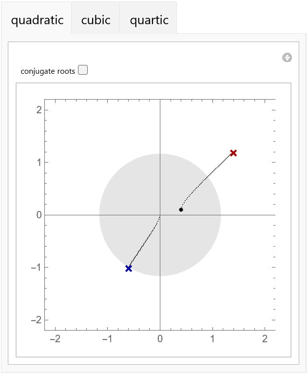
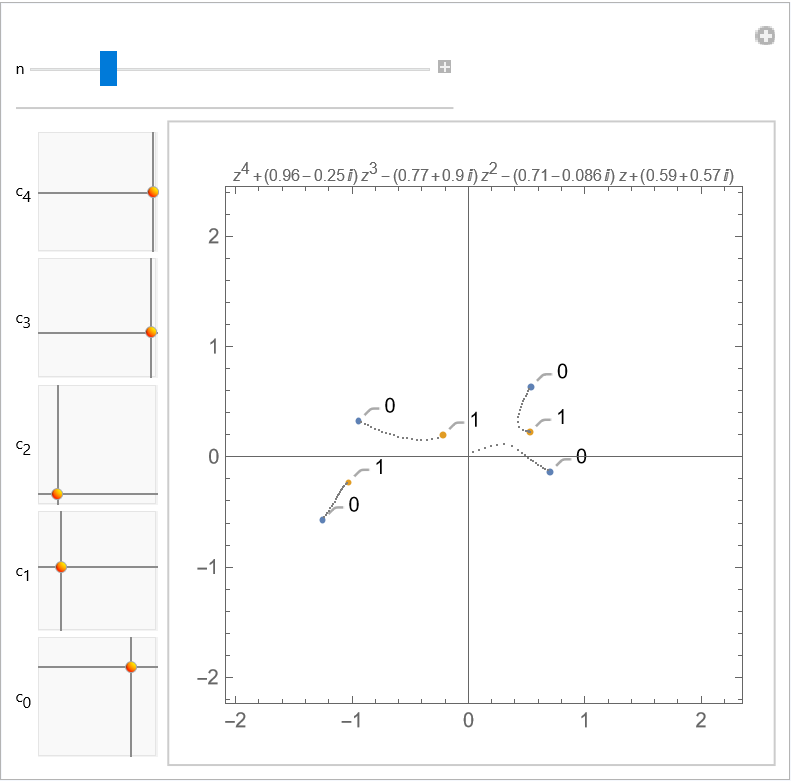
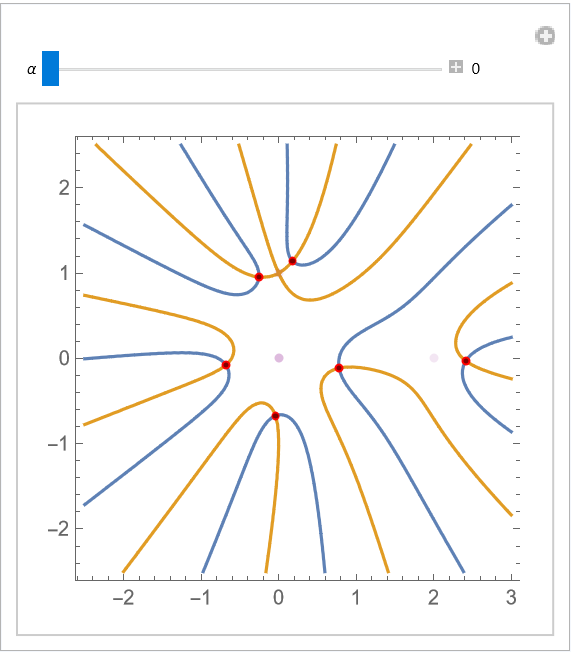
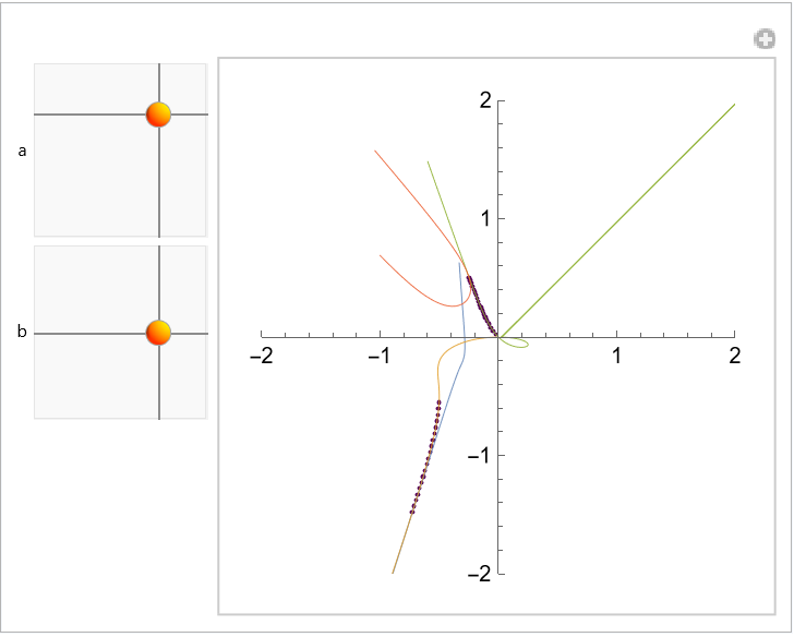
Use these equations to build an interactive demonstration that allows you to move the roots of a quadratic, cubic or quartic polynomial (each root of the defining equation is a Locator, and the dark gray dots represent the fractional derivatives from the interval (0,1)):
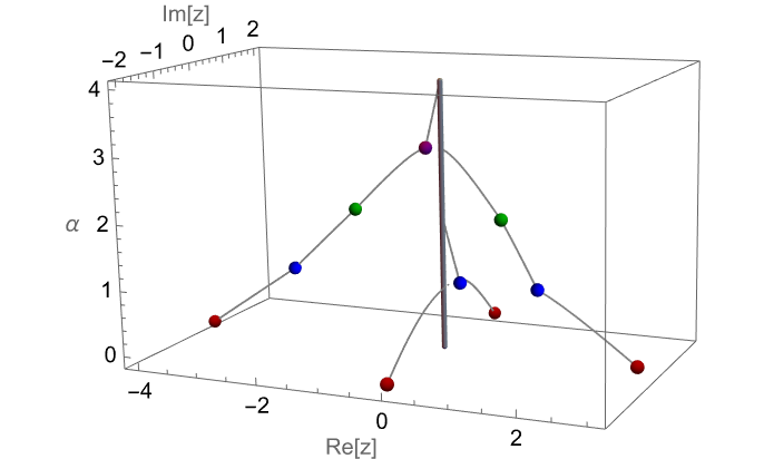
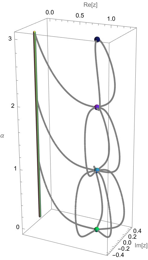
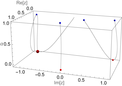
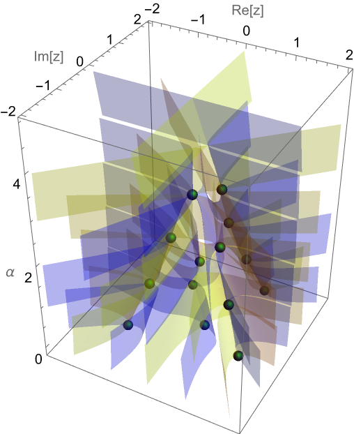
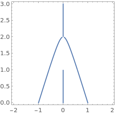
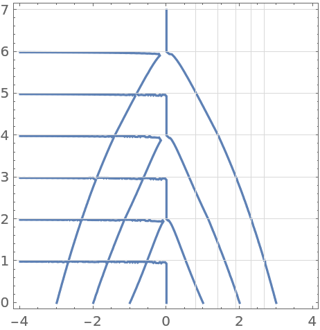
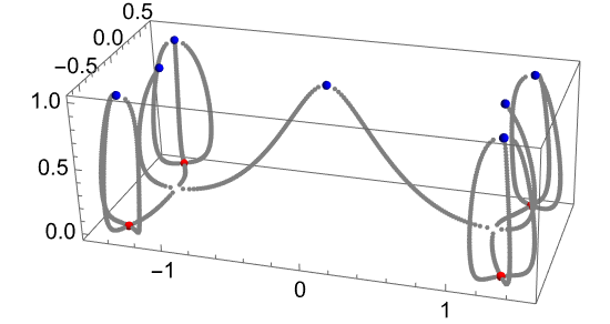
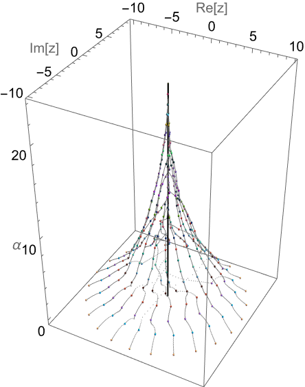
Visualize the movement of the roots of the αth derivative of a quartic polynomial with the derivative order α as a vertical coordinate (the complex conjugate roots ±2i become a real root after differentiation; the gray vertical tube is at the origin of the z plane):
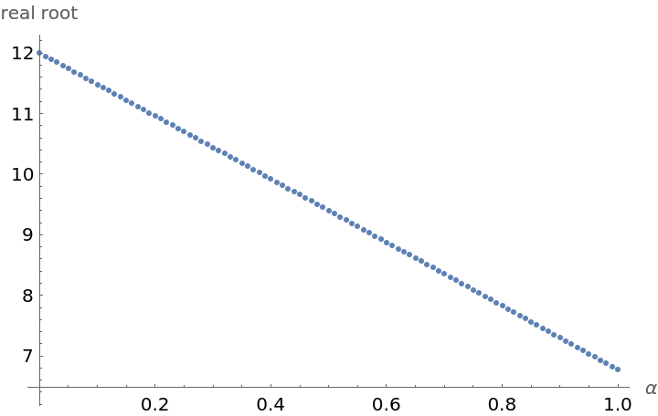
Visualize the movement of the real root from the original cubic polynomial root to the root of the differentiated polynomial:
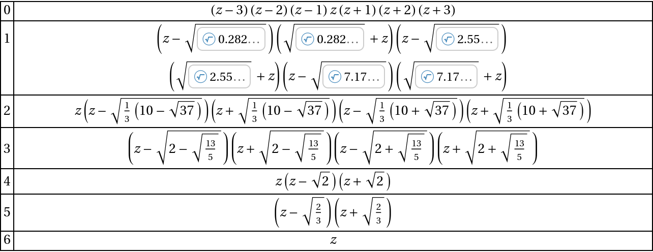
Show the (piecewise-defined) equation that defines the roots' positions as a function of the derivative order α:
Compute the series expansions of these equations for α≈j and α≈j+1:
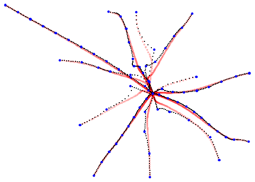
Plot the connection between the roots of a decic polynomial:
Scope (8)
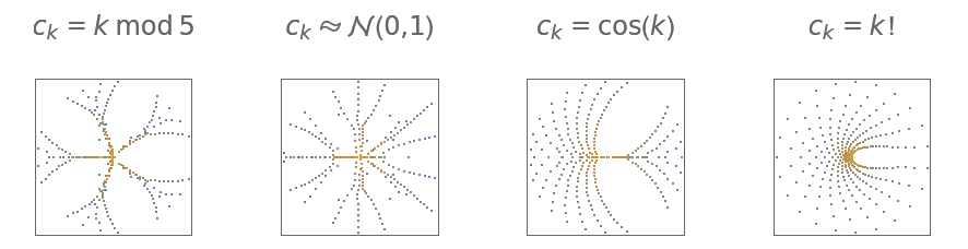
Higher-degree polynomials can be analyzed; here is a polynomial of degree 60 with Gaussian-distributed coefficients:
Plot the roots of integer order in blue and the roots of half-integer order in pink:
The much more symmetrically positioned roots of a polynomial with coefficients ck=k2:
The roots of a polynomial with coefficients ck=sin2(4k):
In all situations, the half-integer-order roots are sandwiched between the integer-order roots.
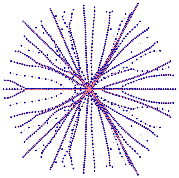
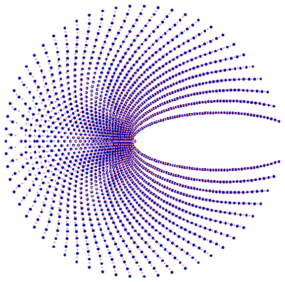
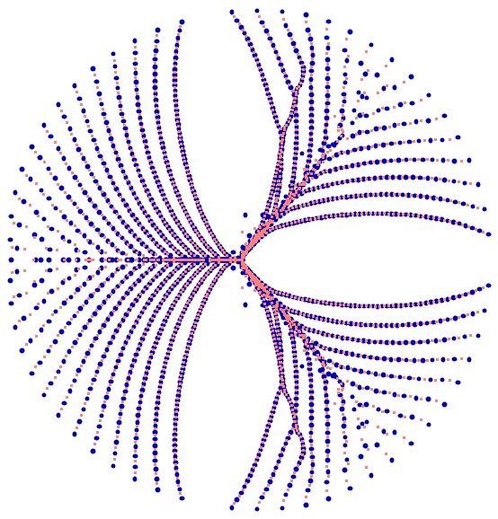
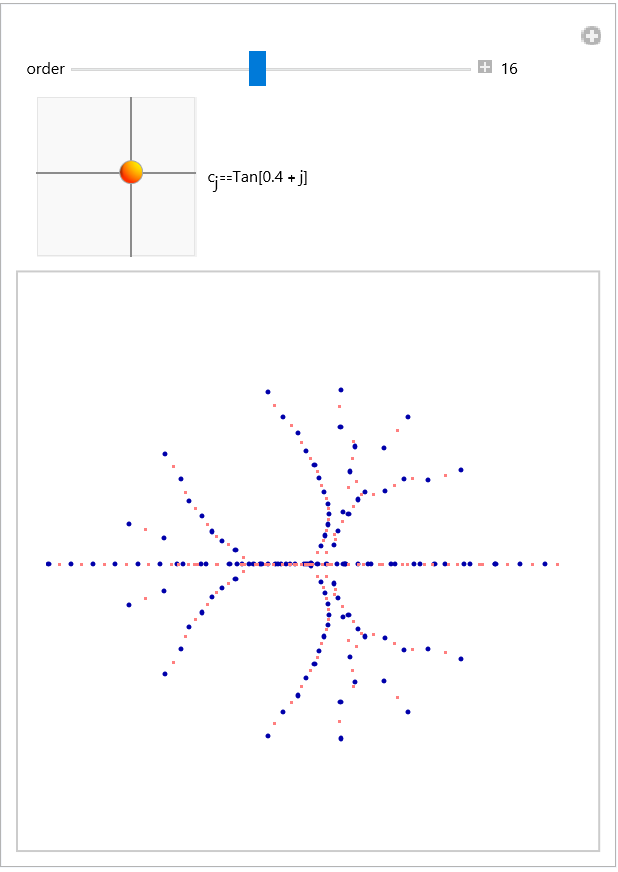
The roots of the polynomials with ck=tan(a+bj) show a rich variety of shapes as functions of a and b:
Plot the roots of higher multiplicity; for each integer-order differentiation, one root migrates to the origin due to the 1/(j-α)! term in the α-range j≤α<j+1 (the vertical tube indicates the origin of the complex z plane):
The (piecewise-defined) equation for the roots of a polynomial fractional-order differentiated polynomial:
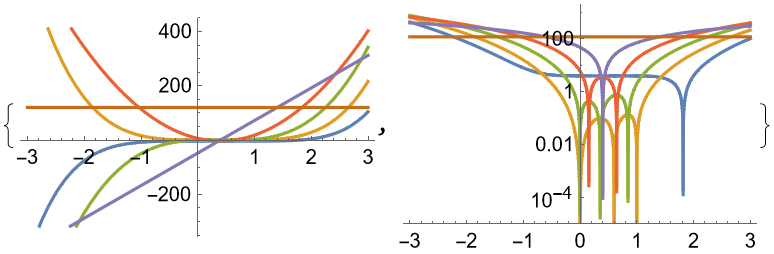
A plot and a log plot of the polynomial and its integer derivatives:
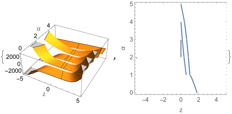
Plot the left-hand side of the first polynomial of the derivative over the z, α plane and mark the real solutions of the equation:
Plot the roots of a quantic polynomial with a triple root at z=-ⅈ as a function of α:
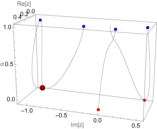
Plotting the roots in 3D as a function of α shows how the triple root splits in a double root and one root that drops out:
Keeping the triple root at z=-ⅈ but moving the other roots closer to the origin shows the split of the triple root into a double root and a single root:
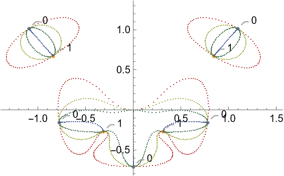
The fractional differentiation order α can be a complex number. The next graphic shows the root curves as a function of α as α goes from 0 to 1 along a curve of the form α(ω)=1/2+(1/2cos(ω)+ⅈhsin(ω)) for π≤ω<2π for various h:
Explore the root paths for a generic quartic polynomial:
Investigate Vieta's formulas for noninteger differentiation order:
The sums of the products of roots for the original and the differentiated polynomial:
The sums of the products of roots for the noninteger-times differentiated polynomial seem to lie on the lines connecting the two point sets:
Check numerically the maximal distance of the fractional-order sums of root products from the line connecting the 0th- and 1st-order points:
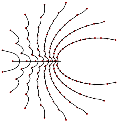
The fractional derivative of a generic degree-12 polynomial for 0≤α<1:
See the structure of the fractional derivative by making the coefficients of the polynomial explicit polynomials in the ck and α:
RootEquation (9)
Obtain the defining equation for the simplest quadratic polynomial:
Solve for the roots of the fractionally differentiated polynomial and simplify the result:
Plot the two roots as a function of α:
Get the equation that determines the roots of a fractionally differentiated sextic:
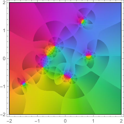
Plot the curves of the vanishing real and imaginary parts and their intersections (the roots) as a function of α for the transition from the polynomial to the differentiated polynomial:
The polynomial equation that defines the fractional roots of a quintic:
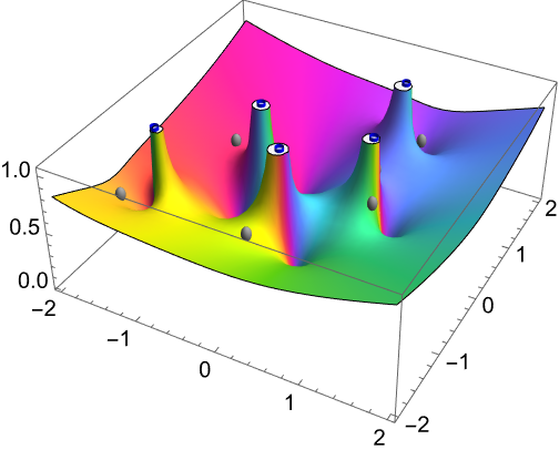
For the α intervals between integers, plot the surfaces of vanishing real and imaginary parts over the complex z plane:
Display the integer derivative roots as spheres together with the surfaces:
Plot the roots of a cubic polynomial:
Compute the equation defining the fractional derivatives:
Compute series solutions for the roots for α≈0 and α≈1:
Compute the asymptotic solution for small α at a double root of a cubic:
At the root with multiplicity 2, one has 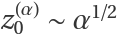 :
:
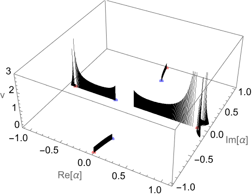
Plot the "speed" of the roots as a function of α for a septic polynomial:
Define the speed as 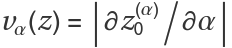 , where
  is a 0 for the fractional derivative order α:
Plot the speeds (the initial speed at a 0 with multiplicity m diverges as vα(z)∼α1/m ):
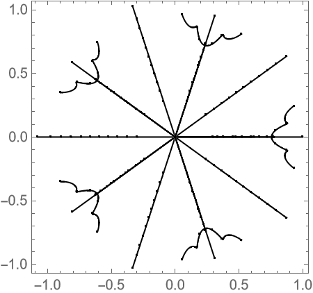
The defining equation of a simple cubic polynomial with three real roots:
Plot the roots of the fractional derivative as a function of α (for this cubic, all roots are always real-valued):
Derive a differential equation for z(α) by differentiation of the defining equation for the range 0≤α<1:
Solve the differential equation numerically:
Plot the differential equation solution together with the previous contour plot:
A septic polynomial with seven real roots:
All 0s of the derivatives are also real:
Use ContourPlot to plot the roots of the fractionally differentiated polynomial:
Compute the defining equation for the roots for a degree-12 polynomial:
Single out the piece that applies to the α range 0≤α<1:
Plot the roots of the fractionally differentiated polynomial for 0<α<12 together with the roots of the singled-out equation outside its range of validity to show that the first equation's roots are globally quite similar to the exact roots:
InterpolatingFunctions (5)
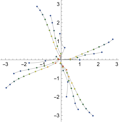
A degree-12 polynomial with roots along a spiral-shaped curve:
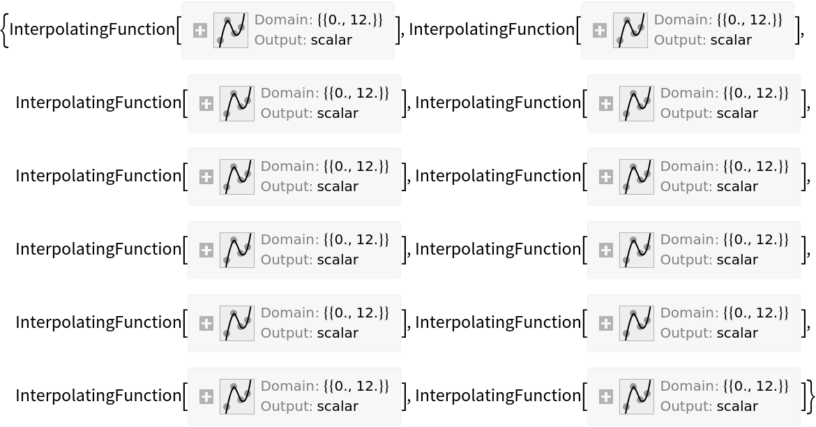
The interpolating functions describing the movements of the roots in the complex plane:
Plot the interpolating functions in the complex plane together with points marking the integer-order derivatives:
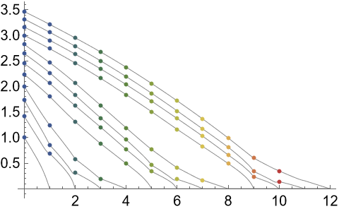
Plot the absolute value of the roots as a function of α showing that at each integer α one root "disappears" at the origin:
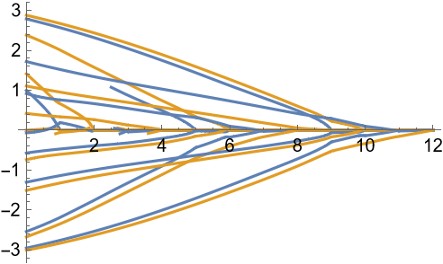
Plot the real and imaginary parts of all roots:
RootConnectingCurves (3)
Visualize the curves connecting the integer roots for the polynomial 1+z+z2+…+z16:
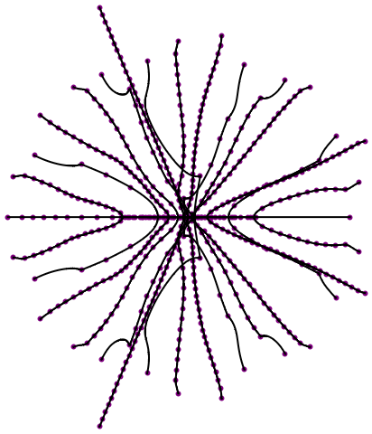
Form a degree-32 polynomial with Gaussian-distributed coefficients:
Compute the roots and root connections:
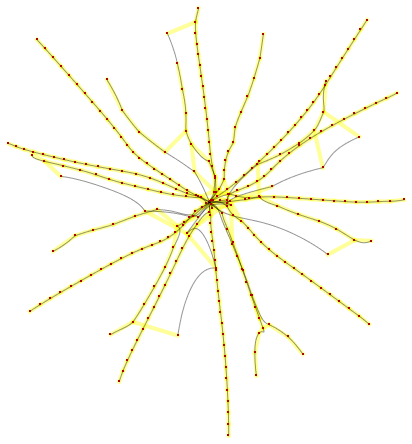
Plot the roots and their connections:
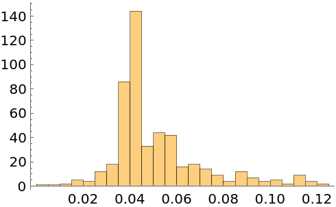
Show a histogram of the distribution of the lengths of the curve segments connecting roots:
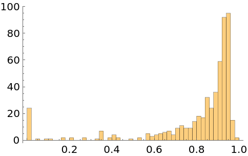
Show a histogram of the ratios of the absolute magnitudes of successive integer-order roots along "root curves":
Form a degree-24 polynomial with Gaussian-distributed complex coefficients:
Compute the roots and root connections:
Compute the shortest connections between the roots of order j and order j+1:
Show the root connections from fractional differentiation and from nearest successive roots together (often, the shortest connection connects the same roots as the root-connecting curves):
RootPathODE (4)
Compute the differential equation for the fractional-order roots of a generic quadratic polynomial:
Simplify the ODE:
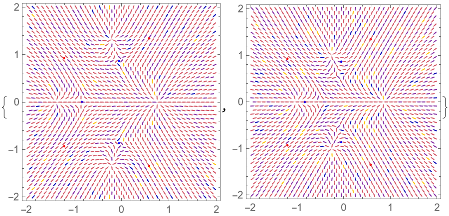
Compute the ODE that governs the root movements from a given sextic polynomial to the roots of its derivative:
The flow field for the root flow at α=0:
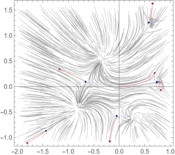
Visualize the flow over the complex z plane:
Plot the absolute magnitude of the flow field together with the positions of the roots of the polynomial and its derivative:
The roots of the derivative are the blue tubes that coincide with the singularities of the flow field for α=0:
Compute again the ODE that governs the root movements from a given sextic polynomial to the roots of its derivative:
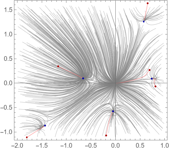
Visualize the flow of random points (not only the 0s) of the z plane under the flow field for the roots:
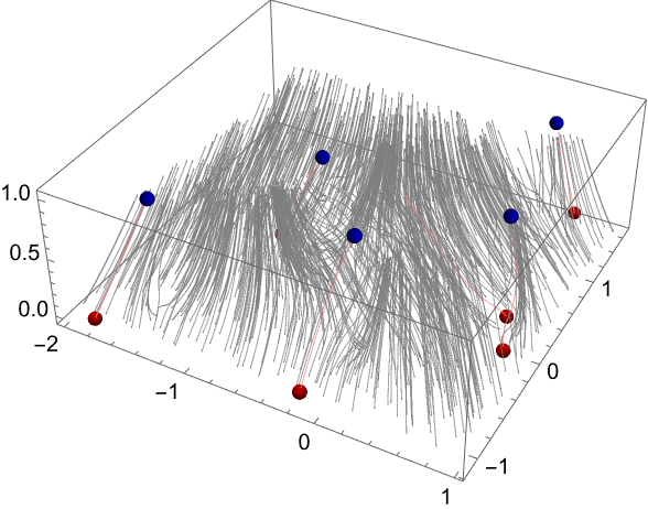
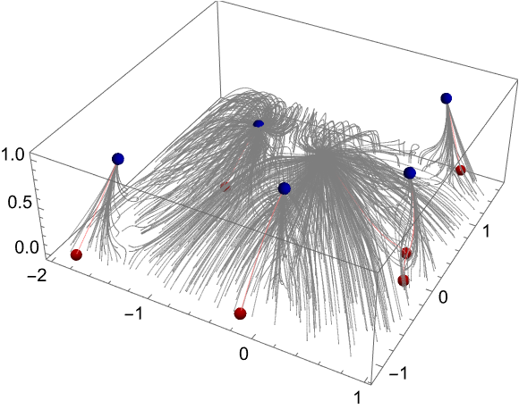
Show the curves in 3D:
Compute again the ODE that governs the movements of any point of the complex z plane from a given sextic polynomial (c is the value of the polynomial at the given point):
Visualize the canonical flow of random points (not only the 0s) of the z plane under the flow field for any point (the value of poly×(-α)! stays constant along each integral curve):
Plotting the curves in 3D shows the overall contractive nature of the flow generated by fractional differentiation (not only the 0s "disappear" at the origin at an integer order of differentiation, and many curves end at the origin):
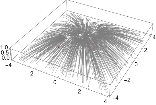
Repeat the last computation for a larger set of start values:
DiscreteRootGraphic and MouseoverGraphic (2)
Get a quick view of the roots of a multiple-times differentiated polynomial with circles indicating the smallest (in magnitude) roots of a given order:
Obtain a graphic with the flow of the roots made interactively visible order by order by mousing over the curve segments:
Applications (8)
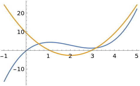
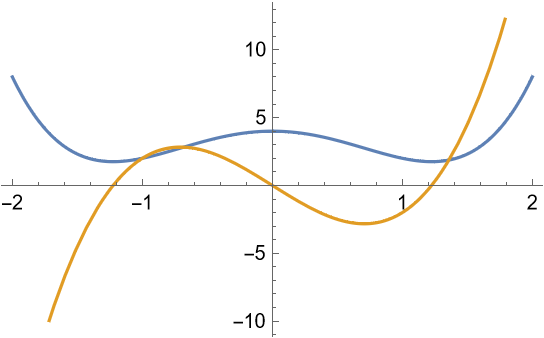
A cubic polynomial with one real root:
The cubic curve has a local maximum and a local minimum, so that derivative has two real roots:
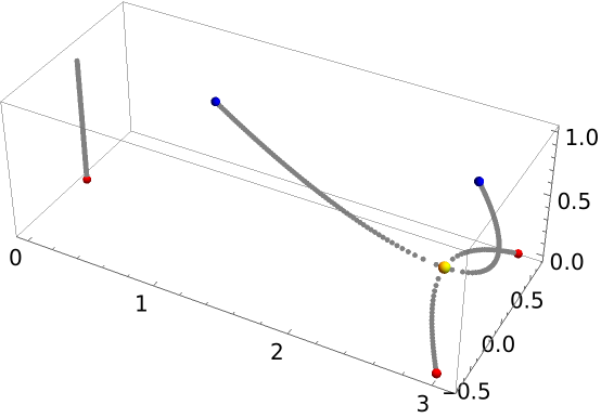
Visualize how the two real roots arise from two complex conjugate roots of the cubic:
Determine the saddle points where the two complex conjugate roots become real by finding where the α-dependent polynomial has a double root (meaning the polynomial and its first derivative have a coinciding root):
Add a yellow sphere indicating the special point:
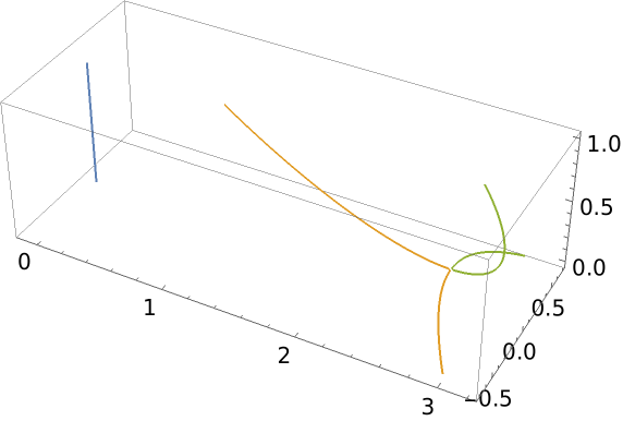
Solve the equation exactly and plot the solutions:
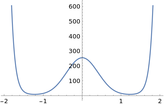
Show how the derivative of a quartic double-well curve with no real roots develops three real roots:
Show how roots with multiplicity develop under fractional differentiation:
Plot the largest by magnitude root over the complex α plane:
Define a cubic with two complex conjugate roots:
Simplify the differential equation for the roots for the α range 0≤α<1:
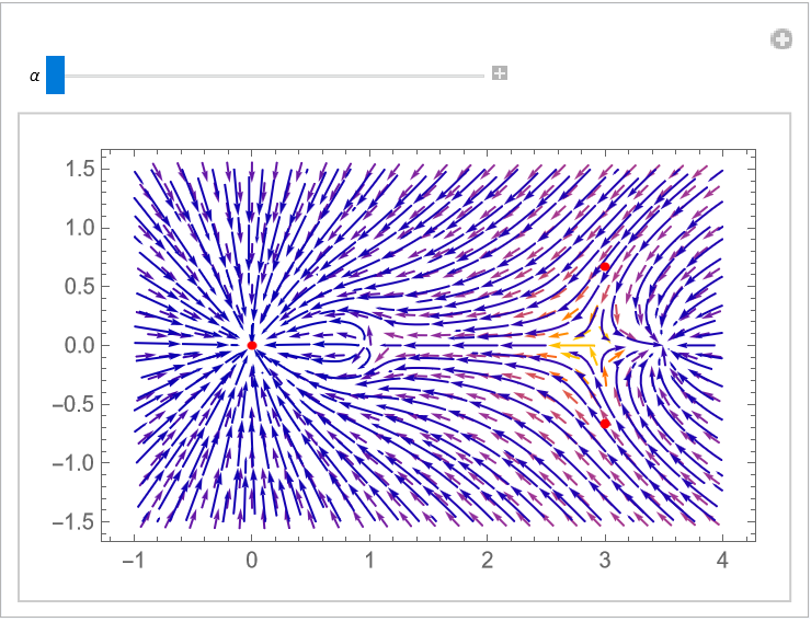
Visualize the trajectories of the roots induced by the root flow field:
Make a contour plot of equi-direction surfaces:
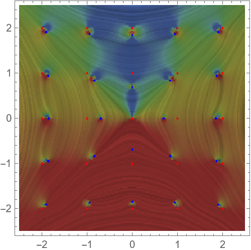
Define a polynomial with roots at the points of a square lattice and the corresponding root flow field:
Visualize the flow field using ListLineIntegralConvolutionPlot:
Visualize the flow field of the roots from an integer to the next integer order for a simple polynomial:
Compute the right-hand side of the differential equation that governs the flow of the roots:
Expand the right-hand side at α=0 and α=1:
Show the vector field in the complex plane:
Obtain the equation for the roots of the fractional derivative with explicit α-dependent coefficients:
Eliminate α to obtain an implicit first-order differential equation q(z(α),z′(α))⩵0:
Eliminate α and z′(α) to obtain an implicit second-order differential equation q(z(α),z″(α))⩵0:
Compute the corresponding initial conditions:
Compare the differential equation solutions with the roots obtained from solving the polynomial directly:
Using z2+az+b=(z-z1)(z-z2), rewrite the equations of motion for the roots in terms of the roots of the initial polynomial rather than the coefficients:
Neat Examples (7)
The root-connecting curves of a degree-20 polynomial:
Define points on a hexagonal lattice:
The corresponding sparse polynomial that uses the points as roots:
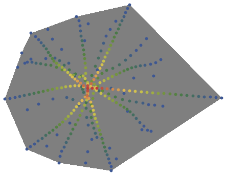
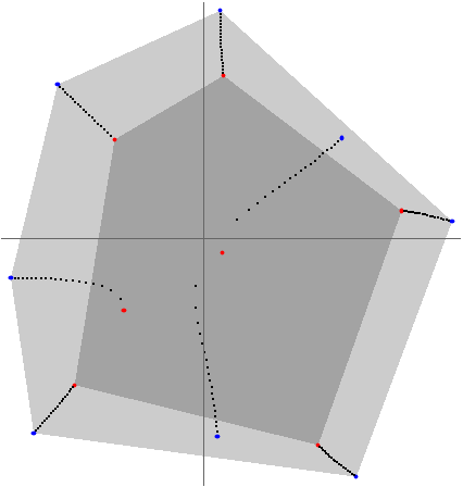
Compute the roots of the fractionally differentiated polynomial and the associated Voronoi meshes:
Interactively modify the differentiation order and visualize the associated Voronoi mesh:
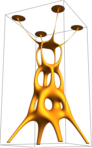
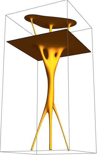
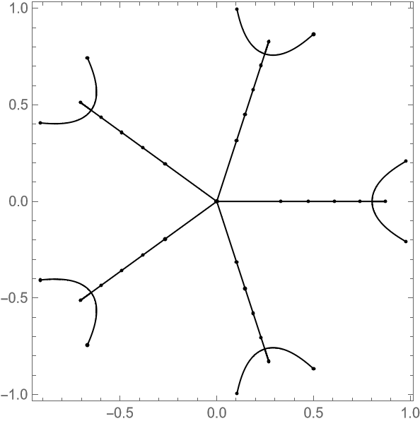
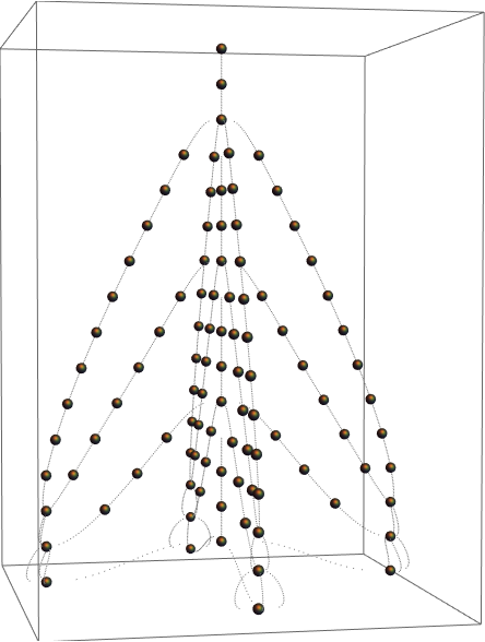
Plot a fractional root church by using a polynomial with roots of high multiplicity:
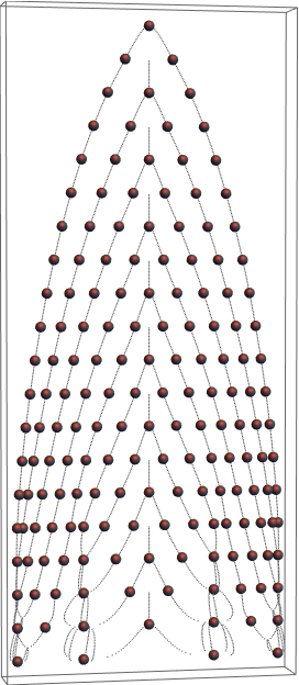
Plot a fractional root tree by using a polynomial with roots of high multiplicity:
Plot a another root tree:
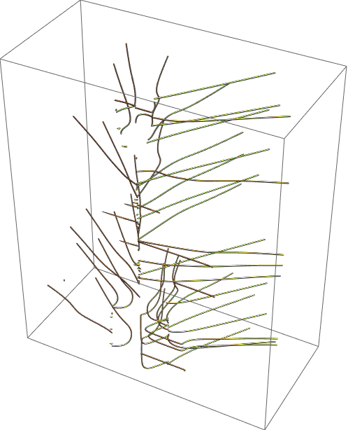
Plot integral curves of the root flow for fizzed values of α:
Define a function that plots the equi-surfaces of finite value c for the equation defining the fractional roots for 0≤α<1:
Plot the surfaces for a cubic and a quartic polynomial:


![ListPlot[{Callout[#, 0] & /@ ReIm[N[z /. Solve[poly == 0, z]]], Callout[#, 1] & /@ ReIm[N[z /. Solve[D[poly, z] == 0, z]]]}, PlotStyle -> (Directive[PointSize[0.02], #] & /@ {Red, Blue})]](https://www.wolframcloud.com/obj/resourcesystem/images/8b2/8b2ae7fa-5c1e-4db6-af4e-650e1e7b5243/4f160ca1f0a412ed.png)
![Show[{%, Graphics[{PointSize[0.01], Gray, PointSize[0.005], Point[ReIm[
N[Flatten[
z /. ResourceFunction["FractionalDPolynomialRoots"][{poly, z}, Range[0.05, 0.95, 0.05]]]]]]}]}]](https://www.wolframcloud.com/obj/resourcesystem/images/8b2/8b2ae7fa-5c1e-4db6-af4e-650e1e7b5243/6aaf5deb837f289e.png)

![Manipulate[
Module[{poly = eq\[Alpha][x + I y, \[Alpha], {a . {1, I}, b . {1, I}}]},
ContourPlot[{Re[poly] == 0, Im[poly] == 0}, {x, -2, 2}, {y, -2, 2},
PerformanceGoal -> "Quality", Axes -> True,
Epilog -> {PointSize[0.02], Point[ReIm[x /. Solve[(poly /. y -> 0) == 0, x]]]}]],
{{\[Alpha], 0}, 0, 1 - 10^-6, Appearance -> "Labeled"},
{{a, {1, 0}}, {-2, -2}, {2, 2}},
{{b, {0, 1}}, {-2, -2}, {2, 2}},
ControlPlacement -> {Top, Left, Left}]](https://www.wolframcloud.com/obj/resourcesystem/images/8b2/8b2ae7fa-5c1e-4db6-af4e-650e1e7b5243/61bcdde42121f169.png)


![TabView[{"quadratic" -> Manipulate[If[cr === True,
Which[r1 =!= Part[aux, 1], r2 = r1 {1, -1}, r2 =!= Part[aux, 2], r1 = r2 {1, -1}, r1 =!= r2 {1, -1}, r2 = r1 {1, -1}]]; aux = {r1, r2}; Module[{poly = (z - Dot[r1, {1, I}]) (z - Dot[
r2, {1, I}])},
Graphics[{
GrayLevel[0.9],
Disk[{0, 0},
Min[
Norm[r1],
Norm[r2]]],
PointSize[0.001],
Darker[Red],
Point[
ReIm[
N[
ReplaceAll[z,
Solve[poly == 0, z]]]]],
PointSize[0.016], Black,
Point[
ReIm[
N[
ReplaceAll[z,
Solve[D[poly, z] == 0, z]]]]],
PointSize[0.01],
GrayLevel[0.3],
PointSize[0.006],
Point[
ReIm[
N[
Flatten[
ReplaceAll[z,
FractionalDPolynomialRoots[{poly, z},
Range[0.02, 0.98, 0.02]]]]]]],
Locator[
Dynamic[r1],
Style["*",
Darker[Red], Bold, 16]],
Locator[
Dynamic[r2],
Style["*",
Darker[Blue], Bold, 16]]}, PlotRange -> 2.2, Axes -> True, Frame -> True]], {{cr, False, "conjugate roots"}, {True, False}}, {{r1, {1.4, 1.2},
Subscript["r", 1]}, {-2, -2}, {2, 2}, ControlType -> None}, {{r2, {-0.6, -1.},
Subscript["r", 2]}, {-2, -2}, {2, 2}, ControlType -> None}, {aux, {{
1.4, 1.2}, {-0.6, -1.2}}, ControlType -> None}, ControlPlacement -> {Top, Left, Left}, TrackedSymbols :> {cr, r1, r2}],
"cubic" -> Manipulate[If[cr === True,
Which[r1 =!= Part[aux, 1], r2 = r1 {1, -1}, r2 =!= Part[aux, 2], r1 = r2 {1, -1}, r1 =!= r2 {1, -1}, r2 = r1 {1, -1}]]; aux = {r1, r2}; Module[{poly = ((z - Dot[r1, {1, I}]) (z - Dot[
r2, {1, I}])) (z - Dot[r3, {1, I}])},
Graphics[{
GrayLevel[0.9],
Disk[{0, 0},
Min[
Norm[r1],
Norm[r2],
Norm[r3]]],
PointSize[0.001],
Darker[Red],
Point[
ReIm[
N[
ReplaceAll[z,
Solve[poly == 0, z]]]]],
PointSize[0.016], Black,
Point[
ReIm[
N[
ReplaceAll[z,
Solve[D[poly, z] == 0, z]]]]],
PointSize[0.01],
GrayLevel[0.3],
PointSize[0.006],
Point[
ReIm[
N[
Flatten[
ReplaceAll[z,
FractionalDPolynomialRoots[{poly, z},
Range[0.02, 0.98, 0.02]]]]]]],
Locator[
Dynamic[r1],
Style["*",
Darker[Red], Bold, 16]],
Locator[
Dynamic[r2],
Style["*",
Darker[Blue], Bold, 16]],
Locator[
Dynamic[r3],
Style["*",
Darker[Green], Bold, 16]]}, PlotRange -> 2.2, Axes -> True, Frame -> True]], {{cr, False,
Row[{"conjugate roots(",
Style["*",
RGBColor[
Rational[2, 3], 0, 0], Bold, 12], " and ",
Style["*",
RGBColor[0, 0,
Rational[2, 3]], Bold, 12], ")"}]}, {True, False}}, {{r1, {1.4, 1.2}, "r"}, {-2, -2}, {2, 2}, ControlType -> None}, {{r2, {-0.6, -1.2}, "r"}, {-2, -2}, {2, 2},
ControlType -> None}, {{r3, {0.4, 0.5}, "r"}, {-2, -2}, {2, 2}, ControlType -> None}, {aux, {{1.4, 1.2}, {-0.6, -1.2}}, ControlType -> None}, ControlPlacement -> {Top, Left, Left}, TrackedSymbols :> True], "quartic" -> Manipulate[If[cr === True,
Which[r1 =!= Part[aux, 1], r2 = r1 {1, -1}, r2 =!= Part[aux, 2], r1 = r2 {1, -1}, r1 =!= r2 {1, -1}, r2 = r1 {1, -1}]]; If[
cr2 === True,
Which[r3 =!= Part[aux, 3], r4 = r3 {1, -1}, r4 =!= Part[aux, 4], r3 = r4 {1, -1}, r3 =!= r4 {1, -1}, r4 = r3 {1, -1}]]; aux = {r1, r2, r3, r4}; Module[{poly = (((z - Dot[r1, {1, I}]) (z - Dot[
r2, {1, I}])) (z - Dot[r3, {1, I}])) (z - Dot[r4, {1, I}])},
Graphics[{
GrayLevel[0.9],
Disk[{0, 0},
Min[
Norm[r1],
Norm[r2],
Norm[r3],
Norm[r4]]],
PointSize[0.001],
Darker[Red],
Point[
ReIm[
N[
ReplaceAll[z,
Solve[poly == 0, z]]]]],
PointSize[0.016], Black,
Point[
ReIm[
N[
ReplaceAll[z,
Solve[D[poly, z] == 0, z]]]]],
PointSize[0.01],
GrayLevel[0.3],
PointSize[0.006],
Point[
ReIm[
N[
Flatten[
ReplaceAll[z,
FractionalDPolynomialRoots[{poly, z},
Range[0.02, 0.98, 0.02]]]]]]],
Locator[
Dynamic[r1],
Style["*",
Darker[Red], Bold, 16]],
Locator[
Dynamic[r2],
Style["*",
Darker[Blue], Bold, 16]],
Locator[
Dynamic[r3],
Style["*",
Darker[Green], Bold, 16]],
Locator[
Dynamic[r4],
Style["*", Purple, Bold, 16]]}, PlotRange -> 2.2, Axes -> True, Frame -> True]], {{cr, False,
Row[{"conjugate roots(",
Style["*",
RGBColor[
Rational[2, 3], 0, 0], Bold, 12], " and ",
Style["*",
RGBColor[0, 0,
Rational[2, 3]], Bold, 12], ")"}]}, {True, False}, ControlPlacement -> 1}, {{cr2, False,
Row[{"conjugate roots(",
Style["*",
RGBColor[0,
Rational[2, 3], 0], Bold, 12], " and ",
Style["*",
RGBColor[0.5, 0, 0.5], Bold, 12], ")"}]}, {True, False}, ControlPlacement -> 2},
Row[{
Manipulate`Place[1], " ",
Manipulate`Place[2]}], {{r1, {1.4, 1.2}, "r"}, {-2, -2}, {2, 2}, ControlType -> None}, {{r2, {-0.6, -1.2}, "r"}, {-2, -2}, {2, 2},
ControlType -> None}, {{r3, {0.6, -0.5}, "r"}, {-2, -2}, {2, 2},
ControlType -> None}, {{r4, {-0.4, 1}, "r"}, {-2, -2}, {2, 2}, ControlType -> None}, {aux, {{1.4, 1.2}, {-0.6, -1.2}}, ControlType -> None}, ControlPlacement -> {Top}, TrackedSymbols :> True]}]](https://www.wolframcloud.com/obj/resourcesystem/images/8b2/8b2ae7fa-5c1e-4db6-af4e-650e1e7b5243/5fa624bd887e1a5d.png)
![roots = Transpose[{{Darker[Red], Blue, Darker[Green], Purple}, Table[Sphere[
Append[ReIm[#], j] & /@ (z /. Solve[D[poly, {z, j}] == 0, z]), 0.1],
{j, 0, 3}]}];](https://www.wolframcloud.com/obj/resourcesystem/images/8b2/8b2ae7fa-5c1e-4db6-af4e-650e1e7b5243/457fde2c530fcf00.png)
![Graphics3D[{roots, Gray, Tube[{{0, 0, 0}, {0, 0, 4}}, 0.04], PointSize[0.004], Gray,
Table[Point[Append[ReIm[#], \[Alpha]] & /@ (z /. ResourceFunction[
"FractionalDPolynomialRoots"][{poly, z}, \[Alpha]])], {\[Alpha], 0, 4 - 1/100, 1/100}]}, Axes -> True, AxesLabel -> {"Re[z]", "Im[z]", "\[Alpha]"}]](https://www.wolframcloud.com/obj/resourcesystem/images/8b2/8b2ae7fa-5c1e-4db6-af4e-650e1e7b5243/232c13374a207c29.png)
![ListPlot[Table[{\[Alpha], Max[Cases[
Chop[x /. ResourceFunction[
"FractionalDPolynomialRoots"][{poly, x}, \[Alpha]]], _Real]]},
{\[Alpha], 0., 1, 1/100}],
AxesLabel -> {"\[Alpha]", "real root"}]](https://www.wolframcloud.com/obj/resourcesystem/images/8b2/8b2ae7fa-5c1e-4db6-af4e-650e1e7b5243/5f676e18be445edf.png)

![Grid[MapIndexed[{#[[2]], Series[#1[[1]], {\[Alpha], #2[[1]] - 1, 1}], Series[#1[[1]], {\[Alpha], #2[[1]], 1}]} &, re[[1, 1]]] // Simplify,
Dividers -> All, Alignment -> Left] // TraditionalForm](https://www.wolframcloud.com/obj/resourcesystem/images/8b2/8b2ae7fa-5c1e-4db6-af4e-650e1e7b5243/2388e5ca7f8b7af4.png)

![Graphics[{rcc, PointSize[0.01], Point[ReIm[Flatten[
N[ResourceFunction["FractionalDPolynomialRoots"][{poly, z}, "IntegerOrderRootList"]]]]]},
Frame -> True]](https://www.wolframcloud.com/obj/resourcesystem/images/8b2/8b2ae7fa-5c1e-4db6-af4e-650e1e7b5243/4c5b3574eee62ef4.png)
![SeedRandom[222];
poly = Sum[RandomVariate[NormalDistribution[0, 1]] z^k, {k, 0, 60}];
Short[poly, 3]](https://www.wolframcloud.com/obj/resourcesystem/images/8b2/8b2ae7fa-5c1e-4db6-af4e-650e1e7b5243/07c2ce7e5c3aa14c.png)
![rootStar[poly_, z_] := Graphics[{Darker[Blue], PointSize[0.01], Point[ReIm[
Flatten[ResourceFunction[
"FractionalDPolynomialRoots"][{poly, z}, "IntegerOrderRootList"]]]],
Pink, PointSize[0.006], Point[ReIm[
Flatten[z /. ResourceFunction["FractionalDPolynomialRoots"][{poly, z}, Table[k + 1/2, {k, 0, Exponent[poly, z] - 1}]]]]]}]](https://www.wolframcloud.com/obj/resourcesystem/images/8b2/8b2ae7fa-5c1e-4db6-af4e-650e1e7b5243/2c7423242634544f.png)
![Manipulate[
Module[{poly = N@Sum[Tan[c . {j, 1}] z^j, {j, 0, o}]},
Show[rootStar[poly, z], PlotRange -> 1.5]],
{{o, 16, "order"}, 2, 32, 1, Appearance -> "Labeled"},
Row[{Control[{{c, {1, 0.4}, ""}, {-5, -5}, {5, 5}}], " ",
Dynamic[ Row[{
\!\(\*SubscriptBox[\("\<c\>"\), \("\<j\>"\)]\), "\[Equal]", Tan[c . {"j", 1}]}]]}],
TrackedSymbols :> True]](https://www.wolframcloud.com/obj/resourcesystem/images/8b2/8b2ae7fa-5c1e-4db6-af4e-650e1e7b5243/1593d72fc05492ca.png)
![Graphics3D[{Table[{RandomColor[], Sphere[{1, 0, j}, 0.04]}, {j, 0, 3}],
Gray, Table[Function[\[Alpha], Point[ Append[#, \[Alpha]] & /@ ReIm[z /. ResourceFunction[
"FractionalDPolynomialRoots"][{poly, z}, \[Alpha]]]]] /@ \[Alpha]List[[j]], {j, 3}],
GrayLevel[0.4], Specularity[Yellow, 5], Tube[{{0, 0, 0}, {0, 0, 3}}, 0.02]},
Axes -> True, AxesLabel -> {"Re[z]", "Im[z]", "\[Alpha]"}]](https://www.wolframcloud.com/obj/resourcesystem/images/8b2/8b2ae7fa-5c1e-4db6-af4e-650e1e7b5243/0806d3185078d64f.png)

![{Plot[Evaluate[Table[D[poly, {z, j}], {j, 0, 5}]], {z, -3, 3}],
LogPlot[Evaluate[Table[Abs[D[poly, {z, j}]], {j, 0, 5}]], {z, -3, 3},
PlotRange -> {10^-5, All}, MaxRecursion -> 12]}](https://www.wolframcloud.com/obj/resourcesystem/images/8b2/8b2ae7fa-5c1e-4db6-af4e-650e1e7b5243/00efe7aaeecbd64b.png)
![{Plot3D[Evaluate[fdr[[1]]], {z, -5, 5}, {\[Alpha], 0, 5},
Exclusions -> Table[\[Alpha] == j, {j, 5}], MeshFunctions -> {#3 &},
Mesh -> {{0}}, MaxRecursion -> 5, AxesLabel -> {"z", "\[Alpha]", None}],
ContourPlot[Evaluate[fdr], {z, -5, 5}, {\[Alpha], 0, 5}, Exclusions -> Table[\[Alpha] == j, {j, 5}], Contours -> 40,
FrameLabel -> {"z", "\[Alpha]"}]}](https://www.wolframcloud.com/obj/resourcesystem/images/8b2/8b2ae7fa-5c1e-4db6-af4e-650e1e7b5243/22b5ce42c83aa5ad.png)
![Graphics[{PointSize[0.015], Red, Point[ReIm[{1, I, -I}]],
Blue, PointSize[0.01], Point[ReIm[N[%]]],
PointSize[0.008], Gray, Table[Point[
ReIm[N[z /. ResourceFunction[
"FractionalDPolynomialRoots"][{poly, z}, \[Alpha]]]]],
{\[Alpha], 0.05, 0.95, 0.05}]}, PlotRange -> 1.5, Axes -> True, Frame -> True]](https://www.wolframcloud.com/obj/resourcesystem/images/8b2/8b2ae7fa-5c1e-4db6-af4e-650e1e7b5243/1087f08fe8cec148.png)
![Graphics3D[{
Red, Sphere[Append[#, 0] & /@ ReIm[{1, I}], 0.02],
Darker[Red], Sphere[Append[#, 0] & /@ ReIm[{-I}], 0.04],
Blue, Sphere[Append[#, 1] & /@ ReIm[N[droots]], 0.02], Gray, PointSize[0.003], Table[Point[Append[#, \[Alpha]] & /@ ReIm[N[z /. ResourceFunction[
"FractionalDPolynomialRoots"][{poly, z}, \[Alpha]]]]],
{\[Alpha], 0.001, 0.999, 0.001}]},
Axes -> True, AxesLabel -> {"Re[z]", "Im[z]", "\[Alpha]"}, ViewPoint -> {3, 1, 1} ]](https://www.wolframcloud.com/obj/resourcesystem/images/8b2/8b2ae7fa-5c1e-4db6-af4e-650e1e7b5243/1928653d583cf919.png)
![Graphics3D[{
Red, Sphere[Append[#, 0] & /@ ReIm[{1, I}/2], 0.02],
Darker[Red], Sphere[Append[#, 0] & /@ ReIm[{-I}], 0.04],
Blue, Sphere[Append[#, 1] & /@ ReIm[N[droots]], 0.02], Gray, PointSize[0.003], Table[Point[
Append[#, \[Alpha]] & /@ ReIm[N[z /. ResourceFunction[
"FractionalDPolynomialRoots"][{poly, z}, \[Alpha]]]]],
{\[Alpha], 0.001, 0.999, 0.001}]},
Axes -> True, AxesLabel -> {"Re[z]", "Im[z]", "\[Alpha]"} , ViewPoint -> {3, 1, 1}]](https://www.wolframcloud.com/obj/resourcesystem/images/8b2/8b2ae7fa-5c1e-4db6-af4e-650e1e7b5243/52fc577ecde5afa3.png)
![Show[{ListPlot[{Callout[#, 0] & /@ ReIm[N[z /. Solve[poly == 0, z]]], Callout[#, 1] & /@ ReIm[N[z /. Solve[D[poly, z] == 0, z]]]}, PlotStyle -> ( Directive[PointSize[0.02], #] &/{Red, Blue})],
Graphics[{ PointSize[0.004], Table[{ColorData["DarkRainbow"][Abs[h]],
Table[
Point[ReIm[
N[z /. ResourceFunction[
"FractionalDPolynomialRoots"][{poly, z}, 1./2 + (1/2 Cos[\[Omega]] + h I Sin[\[Omega]])]]]], {\[Omega], 1. Pi, 2 Pi, Pi/36}]},
{h, {-1, -0.5, -0.25, 0, 0.25, 0.5, 1}}]}]}, PlotRange -> All]](https://www.wolframcloud.com/obj/resourcesystem/images/8b2/8b2ae7fa-5c1e-4db6-af4e-650e1e7b5243/292998835b21a89b.png)
![Manipulate[
Module[{
poly = c4 . {1, I} z^4 + c3 . {1, I} z^3 + c2 . {1, I} z^2 + c1 . {1, I} z + c0 . {1, I}},
Show[{ListPlot[{Callout[#, 0] & /@ ReIm[N[z /. Solve[poly == 0, z]]], Callout[#, 1] & /@ ReIm[N[z /. Solve[D[poly, z] == 0, z]]]}, PlotStyle -> ( Directive[PointSize[0.02], #] &/{Red, Blue})],
Graphics[{PointSize[0.005], Gray, Table[
Point[ReIm[
N[z /. ResourceFunction[
"FractionalDPolynomialRoots"][{poly, z}, \[Alpha]]]]],
{\[Alpha], 1/n, 1 - 1/n, 1/n}]}]},
PlotRange -> 2, Frame -> True, Axes -> True,
AspectRatio -> 1, PlotLabel -> Style[NumberForm[poly, 2], 8]]],
{{n, 20}, 2, 100, 1},
Delimiter,
{{c4, {1, 0}, Subscript["c", 4]}, {-1, -1}, {1, 1}, ImageSize -> Small},
{{c3, RandomReal[{-1, 1}, 2], Subscript["c", 3]}, {-1, -1}, {1, 1}, ImageSize -> Small}, {{c2, RandomReal[{-1, 1}, 2], Subscript["c", 2]}, {-1, -1}, {1, 1}, ImageSize -> Small},
{{c1, RandomReal[{-1, 1}, 2], Subscript["c", 1]}, {-1, -1}, {1, 1}, ImageSize -> Small},
{{c0, RandomReal[{-1, 1}, 2], Subscript["c", 0]}, {-1, -1}, {1, 1}, ImageSize -> Small},
ControlPlacement -> {Top, Left, Left, Left, Left, Left}
]](https://www.wolframcloud.com/obj/resourcesystem/images/8b2/8b2ae7fa-5c1e-4db6-af4e-650e1e7b5243/0cdaf1df9e7d0ff0.png)
![rootSum[poly_, \[Alpha]_, n_] := With[{roots = z /. ResourceFunction[
"FractionalDPolynomialRoots"][{poly, z}, \[Alpha]]},
Total[Times @@@ Subsets[roots, {n}]]]](https://www.wolframcloud.com/obj/resourcesystem/images/8b2/8b2ae7fa-5c1e-4db6-af4e-650e1e7b5243/08bf05805a476f2d.png)
![Graphics[{Red, Point[ReIm[rs0]], Blue, Point[ReIm[rs1]], Gray, MapIndexed[{Point[#], Text[Style[#2[[1]], Bold, 12, Black], Mean[#]]} &, Transpose[Table[Table[ReIm[rootSum[poly, \[Alpha], n]], {n, 5}],
{\[Alpha], 1/12, 11/12, 1/12}]]]}, PlotRange -> All, Frame -> True, Axes -> True]](https://www.wolframcloud.com/obj/resourcesystem/images/8b2/8b2ae7fa-5c1e-4db6-af4e-650e1e7b5243/785c5cf781047af8.png)
![Table[line = Line[ReIm[{rootSum[poly, 0, 1], rootSum[poly, 1, 1]}]]; Max[Table[RegionDistance[line, ReIm[rootSum[poly, \[Alpha], 1]]],
{\[Alpha], 0, 1, 1/100}]],
{n, 5}]](https://www.wolframcloud.com/obj/resourcesystem/images/8b2/8b2ae7fa-5c1e-4db6-af4e-650e1e7b5243/77d2f3679ffc5888.png)


![Manipulate[
ContourPlot[Evaluate[# == 0 & /@ ReIm[\[Tau][x, y, \[Alpha]]] ],
{x, -2.5, 3}, {y, -2.5, 2.5}, PerformanceGoal -> "Quality", Epilog -> {PointSize[0.02], Directive[Red, Opacity[0.1 + 0.9 (1 - \[Alpha])]], Point[ReIm[z /. N[Solve[poly == 0, z]]]], Directive[Purple, Opacity[0.1 + 0.9 \[Alpha]]], Point[ReIm[z /. N[Solve[D[poly, z] == 0, z]]]],
Opacity[0.5], PointSize[0.012], Black, Point[ReIm[z /. N[Solve[\[Tau][z, 0, \[Alpha]] == 0, z]]]]}],
{{\[Alpha], 0}, 0, 1, Appearance -> "Labeled"}]](https://www.wolframcloud.com/obj/resourcesystem/images/8b2/8b2ae7fa-5c1e-4db6-af4e-650e1e7b5243/54de51dca992202c.png)

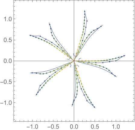
![sliceCP[{p_, Inequality[\[Alpha]1_, LessEqual, Re[\[Alpha]_], Less, \[Alpha]2_]}] := With[{\[CurlyEpsilon] = 10^-8},
ContourPlot3D[Evaluate[{Re[p] == 0, Im[p] == 0} /. z -> x + I y], {x, -2, 2}, {y, -2, 2}, {\[Alpha], \[Alpha]1 + \[CurlyEpsilon], \[Alpha]2 - \[CurlyEpsilon]},
PlotPoints -> {40, 40, 20}, MaxRecursion -> 0,
Mesh -> None, BoundaryStyle -> None,
ContourStyle -> (Directive[Opacity[0.3], #] & /@ {Yellow, Blue}),
AxesLabel -> {"Re[z]", "Im[z]", "\[Alpha]"}]]](https://www.wolframcloud.com/obj/resourcesystem/images/8b2/8b2ae7fa-5c1e-4db6-af4e-650e1e7b5243/4c9af50057931ce2.png)
![roots = Graphics3D[{Directive[GrayLevel[0.2], Specularity[ Darker[Green], 8]],
Table[Sphere[Append[#, j] & /@ N[ReIm[z /. Solve[D[poly, {z, j}] == 0, z]]], 0.1], {j, 0, 3}]}];](https://www.wolframcloud.com/obj/resourcesystem/images/8b2/8b2ae7fa-5c1e-4db6-af4e-650e1e7b5243/53876ab6e8b24900.png)
![Graphics[{PointSize[0.015], Red, Point[ReIm[{1, I, -I}]], Blue, Point[ReIm[N[%]]],
PointSize[0.01], Gray, Table[Point[
ReIm[N[z /. ResourceFunction[
"FractionalDPolynomialRoots"][{poly, z}, \[Alpha]]]]],
{\[Alpha], 0.05, 0.95, 0.05}]}, PlotRange -> 1.5, Axes -> True, Frame -> True]](https://www.wolframcloud.com/obj/resourcesystem/images/8b2/8b2ae7fa-5c1e-4db6-af4e-650e1e7b5243/1d2928af4e9c75fa.png)


![Graphics[{PointSize[0.015], Red, Point[ReIm[{1, I}]],
Blue, PointSize[0.01], Point[ReIm[N[%]]],
PointSize[0.008], Gray, Table[Point[
ReIm[N[z /. ResourceFunction[
"FractionalDPolynomialRoots"][{poly, z}, \[Alpha]]]]],
{\[Alpha], 0.05, 0.95, 0.05}]},
PlotRange -> 1.5, Axes -> True, Frame -> True]](https://www.wolframcloud.com/obj/resourcesystem/images/8b2/8b2ae7fa-5c1e-4db6-af4e-650e1e7b5243/605076bc20d812f4.png)


![Graphics3D[{PointSize[0.02], Opacity[0.5],
Blue, Point[
Append[#, 0] & /@ ReIm[z /. Solve[N[D[poly, z]] == 0, z]]],
Red, Point[Append[#, 0] & /@ ReIm[z /. Solve[N[poly] == 0, z]]],
Opacity[1], Black, Thickness[0.001],
Table[Line[{{Re[#], Im[#], 0}, {Re[#], Im[#],
Abs[rootSpeed[#, \[Alpha]]]}}] & /@ (z /. ResourceFunction[
"FractionalDPolynomialRoots"][{poly, z}, \[Alpha]]),
{\[Alpha], 0.004, 0.996, 0.004}]},
BoxRatios -> {1, 1, 0.4}, Axes -> True, PlotRange -> {All, All, {0, 3}},
AxesLabel -> {"Re[\[Alpha]]", "Im[\[Alpha]]", "v"}]](https://www.wolframcloud.com/obj/resourcesystem/images/8b2/8b2ae7fa-5c1e-4db6-af4e-650e1e7b5243/49531987551991e2.png)


![ContourPlot[Evaluate[fdr], {z, -4, 4}, {\[Alpha], 0, 7}, Exclusions -> Table[\[Alpha] \.00 == j, {j, 7}], GridLines -> {{Sqrt[2/3], Sqrt[2], Sqrt[2 + Sqrt[13/5]], Sqrt[(10 + Sqrt[37])/3], Sqrt[(70 + 259/((871 + 54 I Sqrt[591])/7)^(1/3) +
7^(2/3) (871 + 54 I Sqrt[591])^(1/3))/21]}, Range[7]}, GridLinesStyle -> Directive[Thickness[0.001], LightGray]]](https://www.wolframcloud.com/obj/resourcesystem/images/8b2/8b2ae7fa-5c1e-4db6-af4e-650e1e7b5243/1f1e8d27cd848588.png)

![(* Evaluate this cell to get the example input *) CloudGet["https://www.wolframcloud.com/obj/0d4ac4e5-cc36-4610-8e2e-8157fb56708c"]](https://www.wolframcloud.com/obj/resourcesystem/images/8b2/8b2ae7fa-5c1e-4db6-af4e-650e1e7b5243/104d1b9f08b2230e.png)

![ParametricPlot[
Evaluate[ReIm[#[\[Alpha]]] & /@ ifs], {\[Alpha], 0, 13}, PlotStyle -> Directive[Thickness[0.002], Gray],
Epilog -> derivativeRoots, PlotRange -> All]](https://www.wolframcloud.com/obj/resourcesystem/images/8b2/8b2ae7fa-5c1e-4db6-af4e-650e1e7b5243/7e0e461e656fe966.png)
![roots = Table[{ColorData["DarkRainbow"][j/deg], Point[{j, Abs[#]} & /@ (z /. Solve[D[poly, {z, j}] == 0, z])]},
{j, 0, deg - 1}];](https://www.wolframcloud.com/obj/resourcesystem/images/8b2/8b2ae7fa-5c1e-4db6-af4e-650e1e7b5243/389d126d885cf3ec.png)
![curves = ResourceFunction["FractionalDPolynomialRoots"][{poly, z}, "RootConnectingCurves"]; Graphics[{{Darker[Red], Point[ReIm[
Flatten[z /. ResourceFunction["FractionalDPolynomialRoots"][{poly, z}, "IntegerOrderRoots"]]]]},
Black, curves}]](https://www.wolframcloud.com/obj/resourcesystem/images/8b2/8b2ae7fa-5c1e-4db6-af4e-650e1e7b5243/484f889c7a5f92f2.png)
![Graphics[{ {Thickness[0.01], Opacity[0.4], Yellow, nearLines},
{Thickness[0.001], Opacity[1], Black, curves},
{Darker[Red], PointSize[0.006], Point[ReIm[Flatten[roots]]]}}]](https://www.wolframcloud.com/obj/resourcesystem/images/8b2/8b2ae7fa-5c1e-4db6-af4e-650e1e7b5243/352955addfe1ac92.png)


![ComplexPlot[Evaluate[field\[Alpha]0], {z, -2 - 2 I, 2 + 2 I},
ColorFunction -> "CyclicLogAbsArg",
PlotPoints -> 200, Method -> {"RasterSize" -> 400}]](https://www.wolframcloud.com/obj/resourcesystem/images/8b2/8b2ae7fa-5c1e-4db6-af4e-650e1e7b5243/2856e0574cdce85a.png)
![Show[{cp\[Alpha]0, Graphics3D[{Gray, Sphere[Append[ReIm[#], Abs[field\[Alpha]0 /. z -> #] + 0.03], 0.06] & /@ (z /. Solve[N[poly] == 0, z]),
Blue, CapsuleShape[{Append[ReIm[#], 0], Append[ReIm[#], 1.2]}, 0.05] & /@
(z /. Solve[N[D[poly, z]] == 0, z])}]}]](https://www.wolframcloud.com/obj/resourcesystem/images/8b2/8b2ae7fa-5c1e-4db6-af4e-650e1e7b5243/0da5c980c545b3d2.png)
![path[z0_, style_ : Directive[Gray, Opacity[0.6], Thickness[0.002]]] := Module[{nds = NDSolveValue[{ode, z[0] == z0}, z, {\[Alpha], 0, 1}]},
ParametricPlot[
Evaluate[ReIm[nds[\[Alpha]]]], {\[Alpha], 0, nds[[1, 1, 2]]},
PlotStyle -> style][[1]]] // Quiet](https://www.wolframcloud.com/obj/resourcesystem/images/8b2/8b2ae7fa-5c1e-4db6-af4e-650e1e7b5243/6edfeccd8aecc3b7.png)
![With[{M = 1000},
Graphics[{PointSize[0.012], Darker[Red], Point[ReIm[roots[[1]]]],
Darker[Blue], Point[ReIm[roots[[2]]]],
Monitor[
Table[
path[RandomReal[{-2, 1}] + I RandomReal[{-1.1, 1.6}]], {j, 1000}],
ProgressIndicator[j/M]],
path[#, Directive[Pink, Opacity[0.6], Thickness[0.004]]] & /@ roots[[1]]
}, Frame -> True, Axes -> True]]](https://www.wolframcloud.com/obj/resourcesystem/images/8b2/8b2ae7fa-5c1e-4db6-af4e-650e1e7b5243/280514d993ecb658.png)
![path3D[z0_, style_ : Directive[Gray, Opacity[0.6], Thickness[0.002]]] := Module[{nds = NDSolveValue[{ode, z[0] == z0}, z, {\[Alpha], 0, 1}]},
ParametricPlot3D[Evaluate[Append[ReIm[nds[\[Alpha]]], \[Alpha]]], Evaluate[{\[Alpha], 0, nds[[1, 1, 2]]}],
PlotStyle -> style][[1]]] // Quiet](https://www.wolframcloud.com/obj/resourcesystem/images/8b2/8b2ae7fa-5c1e-4db6-af4e-650e1e7b5243/7fb3c34b729fda05.png)
![With[{M = 1000},
Graphics3D[{PointSize[0.012], Darker[Red], Sphere[Append[#, 0] & /@ ReIm[roots[[1]]], 0.05],
Darker[Blue], Sphere[Append[#, 1] & /@ ReIm[roots[[2]]], 0.05],
Monitor[
Table[path3D[RandomReal[{-2, 1}] + I RandomReal[{-1.1, 1.6}]],
{j, 1000}], ProgressIndicator[j/M]],
path3D[#, Directive[Pink, Opacity[0.6], Thickness[0.002]]] & /@ roots[[1]]}, Axes -> True]]](https://www.wolframcloud.com/obj/resourcesystem/images/8b2/8b2ae7fa-5c1e-4db6-af4e-650e1e7b5243/37e909c7a216db62.png)
![path[z0_, style_ : Directive[Gray, Opacity[0.6], Thickness[0.002]]] := Module[{nds = NDSolveValue[{ode /. c -> (poly /. z -> z0), z[0] == z0} , z, {\[Alpha], 0, 1}]},
ParametricPlot[
Evaluate[ReIm[nds[\[Alpha]]]], {\[Alpha], 0, nds[[1, 1, 2]]},
PlotStyle -> style][[1]]] // Quiet](https://www.wolframcloud.com/obj/resourcesystem/images/8b2/8b2ae7fa-5c1e-4db6-af4e-650e1e7b5243/7c9c5a4bdb1ee0d1.png)
![With[{M = 1000}, Graphics[{
Monitor[Table[path[RandomReal[{-2, 1}] + I RandomReal[{-1.1, 1.6}]],
{j, 1000}], ProgressIndicator[j/M]],
path[#, Directive[Pink, Opacity[0.6], Thickness[0.004]]] & /@ roots[[1]],
PointSize[0.012], Darker[Red], Point[ReIm[roots[[1]]]],
Darker[Blue], Point[ReIm[roots[[2]]]]
}, Frame -> True, Axes -> True]]](https://www.wolframcloud.com/obj/resourcesystem/images/8b2/8b2ae7fa-5c1e-4db6-af4e-650e1e7b5243/54514425eed979b0.png)
![path3D[z0_, style_ : Directive[Gray, Opacity[0.6], Thickness[0.002]]] := Module[{nds = NDSolveValue[{ode /. c -> (poly /. z -> z0), z[0] == z0}, z, {\[Alpha], 0, 1}]},
ParametricPlot3D[Evaluate[Append[ReIm[nds[\[Alpha]]], \[Alpha]]], Evaluate[{\[Alpha], 0, nds[[1, 1, 2]]}],
PlotStyle -> style][[1]]] // Quiet](https://www.wolframcloud.com/obj/resourcesystem/images/8b2/8b2ae7fa-5c1e-4db6-af4e-650e1e7b5243/403b112e83726c58.png)
![With[{M = 1000},
Graphics3D[{PointSize[0.012], Darker[Red], Sphere[Append[#, 0] & /@ ReIm[roots[[1]]], 0.05],
Darker[Blue], Sphere[Append[#, 1] & /@ ReIm[roots[[2]]], 0.05], Monitor[Table[
path3D[RandomReal[{-2, 1}] + I RandomReal[{-1.1, 1.6}]],
{j, 1000}], ProgressIndicator[j/M]], path3D[#, Directive[Pink, Opacity[0.6], Thickness[0.002]]] & /@ roots[[1]]}, Axes -> True]]](https://www.wolframcloud.com/obj/resourcesystem/images/8b2/8b2ae7fa-5c1e-4db6-af4e-650e1e7b5243/0689457c67173439.png)
![With[{M = 1000},
Graphics3D[{PointSize[0.012], Darker[Red], Sphere[Append[#, 0] & /@ ReIm[roots[[1]]], 0.05],
Darker[Blue], Sphere[Append[#, 1] & /@ ReIm[roots[[2]]], 0.05], Monitor[Table[path3D[RandomReal[{-4, 4}] + I RandomReal[{-4, 4}]],
{j, 1000}], ProgressIndicator[j/M]], path3D[#, Directive[Pink, Opacity[0.6], Thickness[0.002]]] & /@ roots[[1]]}, Axes -> True]]](https://www.wolframcloud.com/obj/resourcesystem/images/8b2/8b2ae7fa-5c1e-4db6-af4e-650e1e7b5243/0f511d1927d25890.png)

![gr = Graphics3D[
{Red, Sphere[Append[#, 0] & /@ ReIm[N[z /. Solve[poly == 0, z]]], 0.03],
Blue, Sphere[
Append[#, 1] & /@ ReIm[N[z /. Solve[D[poly, z] == 0, z]]], 0.03],
Gray, PointSize[0.01], Table[Point[
Append[#, \[Alpha]] & /@
ReIm[
N[z /. ResourceFunction[
"FractionalDPolynomialRoots"][{poly, z}, \[Alpha]]]]],
{\[Alpha], 0.01, 0.99, 0.01}]}, Axes -> True]](https://www.wolframcloud.com/obj/resourcesystem/images/8b2/8b2ae7fa-5c1e-4db6-af4e-650e1e7b5243/413f90daad266c23.png)

![gr = Graphics3D[
{Red, Sphere[Append[#, 0] & /@ ReIm[N[z /. Solve[poly == 0, z]]], 0.03],
Blue, Sphere[
Append[#, 1] & /@ ReIm[N[z /. Solve[D[poly, z] == 0, z]]], 0.03],
Gray, PointSize[0.01], Table[Point[
Append[#, \[Alpha]] & /@
ReIm[N[
z /. ResourceFunction[
"FractionalDPolynomialRoots"][{poly, z}, \[Alpha]]]]],
{\[Alpha], 0.01, 0.99, 0.01}]}, Axes -> True]](https://www.wolframcloud.com/obj/resourcesystem/images/8b2/8b2ae7fa-5c1e-4db6-af4e-650e1e7b5243/40e5fe68cb4846f0.png)
![gr = Graphics3D[
{Red, Sphere[Append[#, 0] & /@ ReIm[N[z /. Solve[poly == 0, z]]], 0.03],
Blue, Sphere[
Append[#, 1] & /@ ReIm[N[z /. Solve[D[poly, z] == 0, z]]], 0.03],
Gray, PointSize[0.01], Table[Point[
Append[#, \[Alpha]] & /@
ReIm[N[
z /. ResourceFunction[
"FractionalDPolynomialRoots"][{poly, z}, \[Alpha]]]]],
{\[Alpha], Range[0.01, 0.99, 0.01]^2}]}, Axes -> True]](https://www.wolframcloud.com/obj/resourcesystem/images/8b2/8b2ae7fa-5c1e-4db6-af4e-650e1e7b5243/4d96f11dba092b5e.png)

![Manipulate[
StreamPlot[pVec[x + I y, \[Alpha]], {x, -1, 4}, {y, -1.5, 1.5},
VectorPoints -> Fine, AspectRatio -> Automatic, StreamPoints -> Fine,
Epilog -> {Red, PointSize[0.014], Point[ReIm[
z /. ResourceFunction[
"FractionalDPolynomialRoots"][{poly, z}, \[Alpha]]]]},
ImageSize -> 400],
{\[Alpha], 0., 1}]](https://www.wolframcloud.com/obj/resourcesystem/images/8b2/8b2ae7fa-5c1e-4db6-af4e-650e1e7b5243/68e117074419687f.png)
![ContourPlot3D[
arg[x, y, \[Alpha]], {x, -1, 4}, {y, 0, 2}, {\[Alpha], 0, 1},
PlotPoints -> {80, 50, 50} , MaxRecursion -> 0, Contours -> 8, Mesh -> None,
BoxRatios -> Automatic, ContourStyle -> Opacity[0.6],
AxesLabel -> {"Re[z]", "Im[z]", "a"}]](https://www.wolframcloud.com/obj/resourcesystem/images/8b2/8b2ae7fa-5c1e-4db6-af4e-650e1e7b5243/004e5e160bdb4699.png)
![With[{rhs = z'[\[Alpha]] /. Solve[D[ResourceFunction[
"FractionalDPolynomialRoots"][{poly, z}, \[Alpha],
"RootEquation"][[1, 1, 1, 1]] == 0 /. z -> z[\[Alpha]], \[Alpha]], z'[\[Alpha]]][[1]] /. z[\[Alpha]] -> z},
SetDelayed @@ {pVL[z_?NumericQ, \[Alpha]_] , Normalize[ReIm[rhs]]}]](https://www.wolframcloud.com/obj/resourcesystem/images/8b2/8b2ae7fa-5c1e-4db6-af4e-650e1e7b5243/6fabf6015438f57f.png)
![With[{\[Alpha] = 0.01, pp = 81},
ListLineIntegralConvolutionPlot[
Table[pVL[x + I y, \[Alpha]], {y, -2.5, 2.5, 5/pp}, {x, -2.5, 2.5, 5/pp}],
PerformanceGoal -> "Quality", LineIntegralConvolutionScale -> 5,
ColorFunction -> Function[{x, y, vx, vy, n}, ColorData["DarkRainbow"][Cos[ArcTan[vx, vy]/2]]],
ColorFunctionScaling -> False, RasterSize -> 200, DataRange -> {{-2.5, 2.5}, {-2.5, 2.5}},
Epilog -> With[{roots = N[ResourceFunction["FractionalDPolynomialRoots"][{poly, z}, "IntegerOrderRootList"]]},
{PointSize[0.01], Red, Point[ReIm[roots[[1]]]],
Blue, Point[ReIm[roots[[2]]]] }]] // Quiet]](https://www.wolframcloud.com/obj/resourcesystem/images/8b2/8b2ae7fa-5c1e-4db6-af4e-650e1e7b5243/22c9f6287f371156.png)


![VectorPlot[Evaluate[Normalize@ReIm[Normal[#] /. z -> x + I y]],
{x, -2, 2}, {y, -2, 2}, VectorStyle -> Gray, VectorPoints -> 40, Prolog -> {PointSize[0.012], Red, Point[ReIm[roots]], Blue, Point[ReIm[proots]]},
ImageSize -> 300] & /@
{zpa0, zpa1}](https://www.wolframcloud.com/obj/resourcesystem/images/8b2/8b2ae7fa-5c1e-4db6-af4e-650e1e7b5243/1de759729fe4edf0.png)


![Manipulate[
Block[{a = ac . {1, I}, b = bc . {1, I}, z1, z2, nds},
{z1, z2} = (-a + Sqrt[a^2 - 4 b] {-1, 1})/2;
nds = NDSolve[{ode\[Alpha]2 == 0, z[0] == #, z'[0] == (3 b + a #)/(2 (a + 2 #))}, z, {\[Alpha], -2, 2}] & /@ {z1, z2}; ParametricPlot[
Evaluate[ReIm[z[\[Alpha]] /. #] & /@ Flatten[nds]], {\[Alpha], -2,
2},
PlotRange -> 2, PlotStyle -> Thickness[0.002], Prolog -> {Darker[Purple], PointSize[0.01],
Table[
Point[ReIm[
z /. ResourceFunction[
"FractionalDPolynomialRoots"][{z^2 + a z + b, z}, \[Alpha]]]],
{\[Alpha], 0.05, 0.95, 0.05}]}]] // Quiet,
{{ac, {1, 1}, "a"}, {-2, -2}, {2, 2}},
{{bc, {1, 0}, "b"}, {-2, -2}, {2, 2}},
ControlPlacement -> Left]](https://www.wolframcloud.com/obj/resourcesystem/images/8b2/8b2ae7fa-5c1e-4db6-af4e-650e1e7b5243/1d6fb5c650bcb86b.png)

![derivativeRoots = Table[{ColorData["DarkRainbow"][j/deg],
Point[ReIm[z /. Solve[D[poly, {z, j}] == 0, z]]]}, {j, 0, deg - 1}];
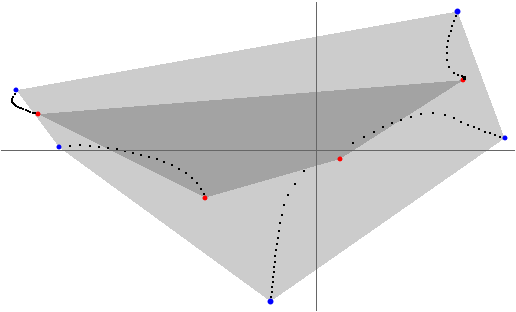
Graphics[{Gray, ConvexHullMesh[derivativeRoots[[1, 2, 1]]], derivativeRoots}]](https://www.wolframcloud.com/obj/resourcesystem/images/8b2/8b2ae7fa-5c1e-4db6-af4e-650e1e7b5243/7d24661770041959.png)
![deg = 8;
SeedRandom[2];
poly = Sum[RandomReal[] Exp[2 Pi I Random[]] z^k, {k, 0, deg}];](https://www.wolframcloud.com/obj/resourcesystem/images/8b2/8b2ae7fa-5c1e-4db6-af4e-650e1e7b5243/4b360ed42cc4d9e5.png)
![Graphics[{Opacity[0.2], ConvexHullMesh[pRoots], ConvexHullMesh[dPRoots],
Opacity[1], PointSize[0.01], Blue, Point[pRoots], Red, Point[dPRoots],
Black, PointSize[0.003], Table[Point[
ReIm[z /. ResourceFunction[
"FractionalDPolynomialRoots"][{poly, z}, \[Alpha]]]],
{\[Alpha], 0.05, 0.95, 0.05}]},
Axes -> True, Ticks -> None]](https://www.wolframcloud.com/obj/resourcesystem/images/8b2/8b2ae7fa-5c1e-4db6-af4e-650e1e7b5243/748eb88a4924c4cb.png)
![Graphics[{Opacity[0.2], ConvexHullMesh[pRoots], ConvexHullMesh[dPRoots],
Opacity[1], PointSize[0.01], Blue, Point[pRoots], Red, Point[dPRoots],
Black, PointSize[0.003],
Table[
Point[ReIm[
z /. ResourceFunction[
"FractionalDPolynomialRoots"][{poly, z}, \[Alpha]]]],
{\[Alpha], 0.05, 0.95, 0.05}]},
Axes -> True, Ticks -> None]](https://www.wolframcloud.com/obj/resourcesystem/images/8b2/8b2ae7fa-5c1e-4db6-af4e-650e1e7b5243/57f814a144836af6.png)
![approximateDRoots[poly_, z_] := Module[{roots, nf, T1, T2, T3},
roots = z /. Solve[poly == 0, z];
T1 = Table[
roots[[j]] -> roots[[j]] - 1/(Total[1/(roots[[j]] - Delete[roots, j])]), {j, Length[roots]}];
T2 = MapAt[0. &, SortBy[T1, Abs[#[[2]]] &], {{1, 2}}];
nf = Nearest[Append[z /. Solve[D[poly, z] == 0, z], 0. I]];
T3 = SortBy[Prepend[(#1 -> nf[#2][[1]]) & @@@ Rest[T2], First[T2]], Abs[#[[1]]] &]]](https://www.wolframcloud.com/obj/resourcesystem/images/8b2/8b2ae7fa-5c1e-4db6-af4e-650e1e7b5243/766a54e38eb930dc.png)


![Graphics[{rcc, PointSize[0.01], Point[ReIm[
Flatten[N[
ResourceFunction["FractionalDPolynomialRoots"][{poly, z}, "IntegerOrderRootList"]]]]]},
Frame -> True]](https://www.wolframcloud.com/obj/resourcesystem/images/8b2/8b2ae7fa-5c1e-4db6-af4e-650e1e7b5243/2f4aba8e140a0970.png)

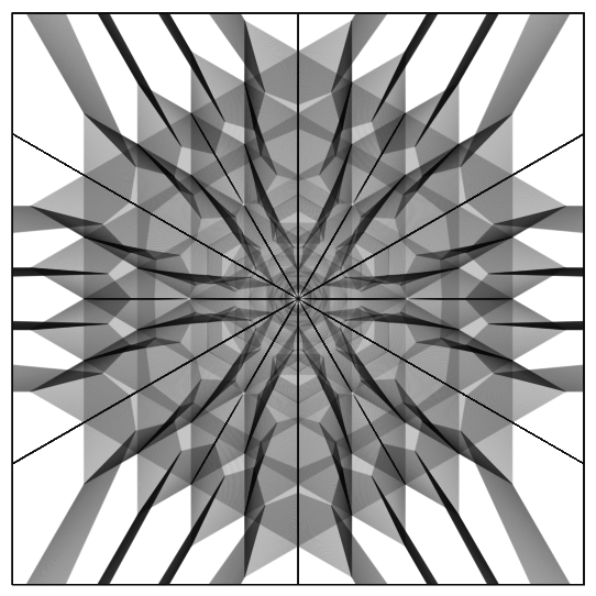
![Graphics[{Thickness[0.001], Opacity[0.1],
Table[MeshPrimitives[ VoronoiMesh[
ReIm[z /. ResourceFunction[
"FractionalDPolynomialRoots"][{poly, z}, \[Alpha]]],
{{-8, 8}, {-8, 8}}], {1}], {\[Alpha], 0, 30, 0.1}]}]](https://www.wolframcloud.com/obj/resourcesystem/images/8b2/8b2ae7fa-5c1e-4db6-af4e-650e1e7b5243/141f4adff46efd17.png)
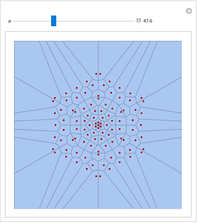
![Manipulate[
With[{L = 8.5, rts = ReIm[
z /. ResourceFunction[
"FractionalDPolynomialRoots"][{poly, z}, \[Alpha]]]}, Show[{VoronoiMesh[rts, {{-L, L}, {-L, L}}], Graphics[{Darker[Red], Point[rts]}]}, PlotRange -> L]],
{{\[Alpha], 0}, 0, 144, Appearance -> "Labeled"}]](https://www.wolframcloud.com/obj/resourcesystem/images/8b2/8b2ae7fa-5c1e-4db6-af4e-650e1e7b5243/2ce9322b6b4736cf.png)
![Graphics3D[{GrayLevel[0.3], Specularity[Red, 12], roots, PointSize[0.003],
Table[Point[Append[ReIm[#], \[Alpha]] & /@ (z /. ResourceFunction[
"FractionalDPolynomialRoots"][{poly, z}, \[Alpha]])],
{\[Alpha], 0, 19 - 1/20, 1/20}]}, Axes -> False, ViewPoint -> {-0.65, -3.32, 0.12}]](https://www.wolframcloud.com/obj/resourcesystem/images/8b2/8b2ae7fa-5c1e-4db6-af4e-650e1e7b5243/4fb31a260d3d1fec.png)
![Graphics3D[{GrayLevel[0.2], Specularity[Orange, 12], roots, PointSize[0.003], Gray,
Table[Point[Append[ReIm[#], \[Alpha]] & /@ (z /. ResourceFunction[
"FractionalDPolynomialRoots"][{poly, z}, \[Alpha]])],
{\[Alpha], 0, 15 - 1/20, 1/20}]}, Axes -> False, ViewPoint -> {-0.65, -3.32, 0.12}]](https://www.wolframcloud.com/obj/resourcesystem/images/8b2/8b2ae7fa-5c1e-4db6-af4e-650e1e7b5243/4fef74779956530e.png)
![roots = Transpose[{RandomColor[deg],
Table[Ellipsoid[#, 0.1 {1, 1, (deg + 1)/22}] & /@ (Append[ReIm[#], j] & /@ (z /. Solve[D[poly, {z, j}] == 0, z])),
{j, 0, deg - 1}]}];](https://www.wolframcloud.com/obj/resourcesystem/images/8b2/8b2ae7fa-5c1e-4db6-af4e-650e1e7b5243/6789a0a20acfc910.png)
![Graphics3D[{roots, {Directive[Black, Specularity[Yellow, 12]], Tube[{{0, 0, 0}, {0, 0, deg}}, 0.08]}, PointSize[0.002], Gray, Table[Point[Append[ReIm[#], \[Alpha]] & /@ (z /. ResourceFunction[
"FractionalDPolynomialRoots"][{poly, z}, \[Alpha]])], {\[Alpha], 0, deg - 1/20, 1/20}]}, Axes -> True, AxesLabel -> {"Re[z]", "Im[z]", "\[Alpha]"}, BoxRatios -> {1, 1, 3/2}]](https://www.wolframcloud.com/obj/resourcesystem/images/8b2/8b2ae7fa-5c1e-4db6-af4e-650e1e7b5243/08281179504575d5.png)
![fixed\[Alpha]IntegralCurve[z0_] := Block[{\[Alpha] = RandomReal[{0, 3}], dir, nds},
dir[z_Complex] = Sign[rhs]; nds = NDSolveValue[{z'[\[Tau]] == dir[z[\[Tau]]], z[0] == z0,
WhenEvent[Abs[z[\[Tau]]] > 1.25, "StopIntegration"]}, z, {\[Tau], -2, 2},
Method -> "Adams", PrecisionGoal -> 4] // Quiet;
Tube[Cases[
Normal[ParametricPlot3D[
Evaluate[{Re[nds[\[Tau]]], Im[nds[\[Tau]]], \[Alpha]}], Evaluate[
Flatten[{\[Tau], nds[[1, 1]]}]]]], _Line, \[Infinity]][[1]], 0.006]]](https://www.wolframcloud.com/obj/resourcesystem/images/8b2/8b2ae7fa-5c1e-4db6-af4e-650e1e7b5243/579a9eae4abbf84e.png)
![With[{m = 100},
Monitor[Graphics3D[{GrayLevel[0.3], Specularity[Yellow, 12],
Table[
fixed\[Alpha]IntegralCurve[
RandomReal[] Exp[2 Pi I RandomReal[]]], {j, m}]}, PlotRange -> {All, {0, All}, All}, BoxRatios -> Automatic],
ProgressIndicator[j/m]]]](https://www.wolframcloud.com/obj/resourcesystem/images/8b2/8b2ae7fa-5c1e-4db6-af4e-650e1e7b5243/469048f0cd7aa50c.png)
![rootEquationPlot3D[{poly_, z_}, \[Alpha]M_, c_] := With[{rh = ResourceFunction[
"FractionalDPolynomialRoots"][{poly, z}, \[Alpha], "RootEquation"][[1, 1, 1, 1]],
L = 1.2 Max[Norm /@ (z /. Solve[poly == 0, z])], pp = 160}, Module[{cf, data},
data = Table[cf = Compile[{x, y}, Evaluate[ComplexExpand[Abs[ rh /. z -> x + I y] ]],
CompilationOptions -> {"ExpressionOptimization" -> True}];
Table[cf[x, y ], {y, -L, L, 2 L/pp}, {x, -L, L, 2 L/pp}],
{\[Alpha], 0., \[Alpha]M - 1/pp, 2/pp}]; ListContourPlot3D[data, Contours -> {c}, Mesh -> None, BoxRatios -> {1, 1, 2},
ViewPoint -> {2, 1, -0.6}, Axes -> False, ImageSize -> 360]
]]](https://www.wolframcloud.com/obj/resourcesystem/images/8b2/8b2ae7fa-5c1e-4db6-af4e-650e1e7b5243/5111cb04c234be23.png)