Wolfram Function Repository
Instant-use add-on functions for the Wolfram Language
Function Repository Resource:
Model ball trajectories in a 2D Galton board using Hertzian force laws between the ball and the pegs
ResourceFunction["GaltonBoardModel"][brd,inits, output] models the dynamics in a Galton board brd with ball initial conditions inits and returns the model result output as the graphic or data. | |
ResourceFunction["GaltonBoardModel"][brd,prop] computes the property prop of the Galton board brd. | |
ResourceFunction["GaltonBoardModel"]["RandomGaltonBoard"] returns a random Galton board. |
| "RowCount" | number of rows of pegs |
| "PegRadius" | radius of the pegs |
| "PegHardness" | hardness of the pegs |
| "PegForceExponent" | exponent of the force law |
| "PegRotation" | rotation of the peg deformation from the radial direction |
| "VerticalAcceleration" | vertical acceleration |
| "LinearFrictionCoefficient" | friction force on the balls proportional to their speed |
| "QuadraticFrictionCoefficient" | friction force on the balls proportional to their speed squared |
| "BallRadius" | radius of the balls |
| xi | assume y=1 and {vx,i,vy,i}={0,0} |
| {xi,yi} | assume {vx,vy}={0,0} |
| {{xi,yi},{vx,i,vy,i}} | fully specified initial conditions |
| "PathGraphics" | a graphic of the pegs and ball paths |
| "PathGraphics3D" | a 3D graphic of the pegs and ball paths with the ball velocities as the z values |
| "Paths" | list of paths as styled line primitives |
| "FinalPosition" | a list of the positions of the balls one unit down from the last row of pegs |
| "PathArcLengths" | a list of the arc lengths of the ball paths |
| "ArrivalTimes" | a list of the arrival times of the ball paths |
| "InterpolatingFunctions" | a list of pairs of {position,velocity} interpolating functions of the ball paths |
| {"PathArrayPlot", dim} | an array plot of dimension dim×dim of the ball path |
| "TimeEvolution" | an interactive demonstration allowing you to step through the ball-falling process |
| "Manipulate" | an interactive demonstration allowing you to change board parameters and ball initial positions |
| "TrajectoryStyle" | {blue,white} | color directive for the ball paths |
| "PegStyle" | slightly opaque dark red | pair of center-boundary colors of the pegs |
| "TotalPegCount" | the total count of pegs |
| "MinPegDistance" | the minimum distance between two pegs |
| "PegPositions" | a list of the center corrdinates of the pegs |
| "ForceLawSketch" | sketch of the specified Hertzian force law |
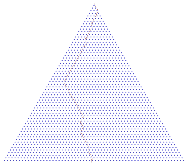
A single ball path in a large Galton board of 60 rows of pegs:
| In[1]:= |
![board = <|
"RowCount" -> 60, "PegRadius" -> 0.25,
"PegHardness" -> 100,
"PegForceExponent" -> 1.25,
"PegRotation" -> 0,
"VerticalAcceleration" -> 1,
"LinearFrictionCoefficient" -> 0.4,
"QuadraticFrictionCoefficient" -> 1,
"BallRadius" -> 0.1|>;
ResourceFunction["GaltonBoardModel"][board, {0.3}, "PathGraphics"]](https://www.wolframcloud.com/obj/resourcesystem/images/895/895a0403-4399-4c3f-b413-14abc3a23f23/633c847e602d1187.png)
|
| Out[2]= |
|
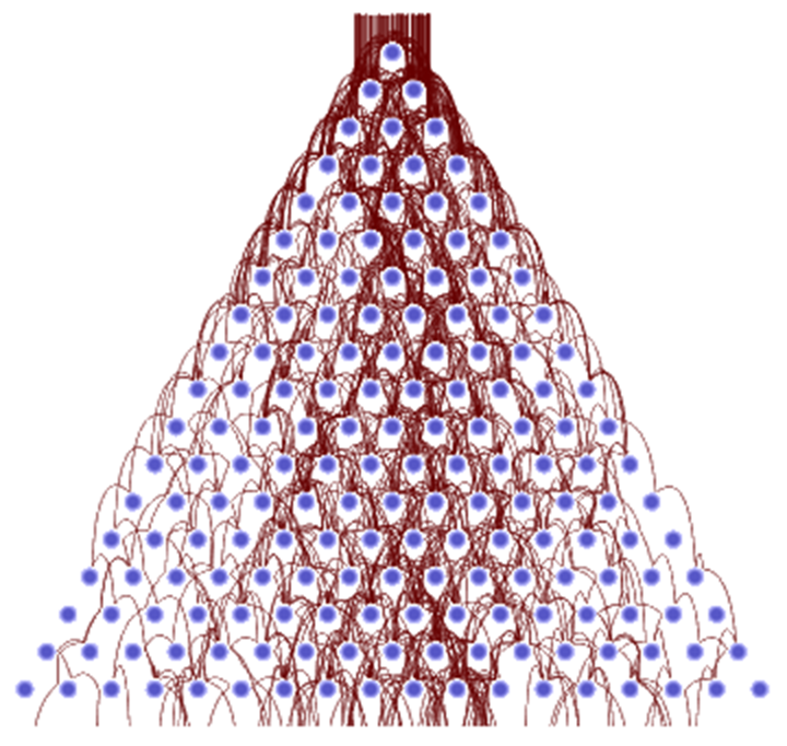
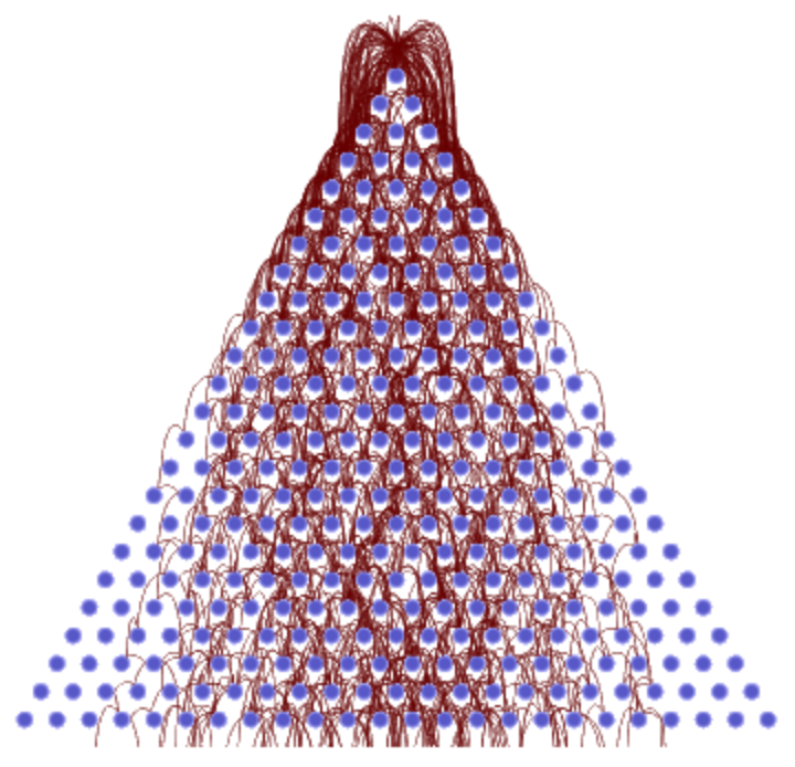
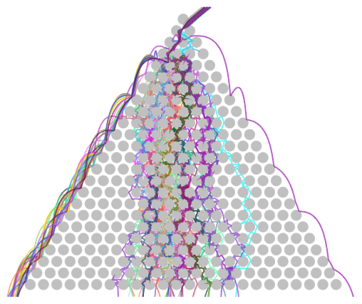
The ball paths for a typically sized Galton board using a realistic force law and finite-sized balls:
| In[3]:= |
![board = <|
"RowCount" -> 18, "PegRadius" -> 0.25, "PegHardness" -> 100,
"PegForceExponent" -> 3/2,
"PegRotation" -> 0,
"VerticalAcceleration" -> 1,
"LinearFrictionCoefficient" -> 0,
"QuadraticFrictionCoefficient" -> 1,
"BallRadius" -> 0.1|>;
ResourceFunction["GaltonBoardModel"][board, Table[{RandomReal[{-1, 1}], 1}, 100], "PathGraphics"]](https://www.wolframcloud.com/obj/resourcesystem/images/895/895a0403-4399-4c3f-b413-14abc3a23f23/392acfa4c09c63ee.png)
|
| Out[3]= |
|
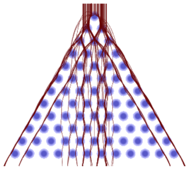
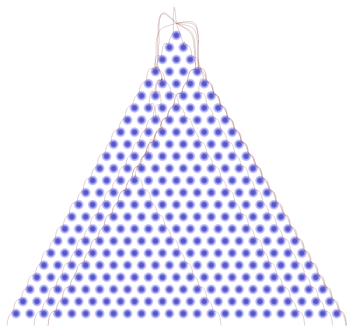
Point-size balls, no friction lead and a small friction coefficient:
| In[4]:= |
![board = <|
"RowCount" -> 12, "PegRadius" -> 0.3, "PegHardness" -> 100,
"PegForceExponent" -> 3/2,
"PegRotation" -> 0,
"VerticalAcceleration" -> 1,
"LinearFrictionCoefficient" -> 0.5,
"QuadraticFrictionCoefficient" -> 0,
"BallRadius" -> 0.|>;
ResourceFunction["GaltonBoardModel"][board, Table[{x, 1}, {x, -1, 1, 2/48}], "PathGraphics"]](https://www.wolframcloud.com/obj/resourcesystem/images/895/895a0403-4399-4c3f-b413-14abc3a23f23/42dce302e7e9628e.png)
|
| Out[4]= |
|
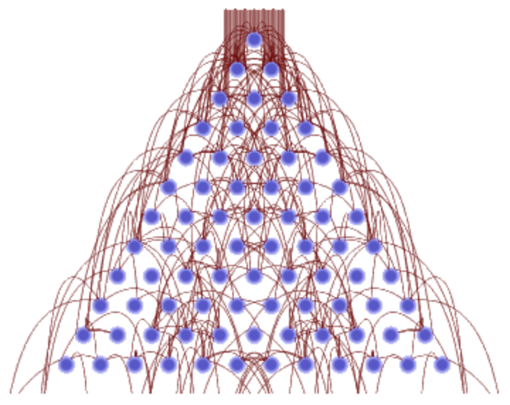
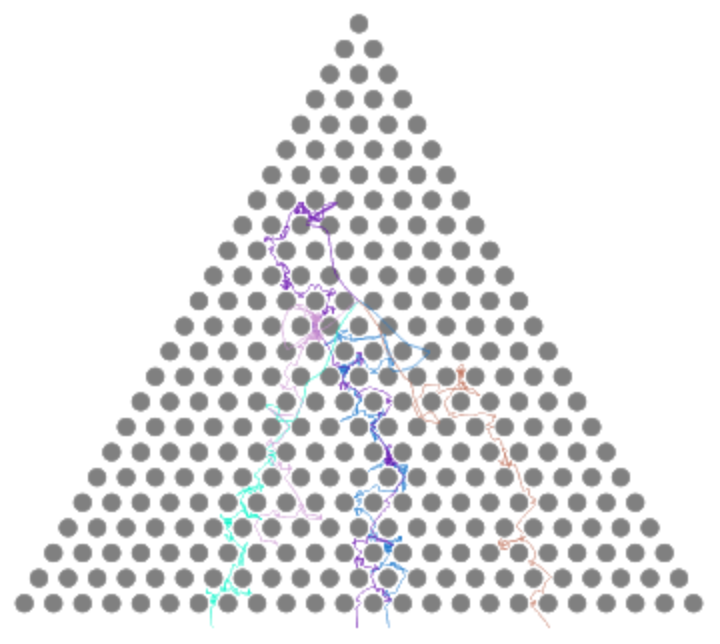
Large, soft pegs allow particles to substantially penetrate and deform the pegs:
| In[5]:= |
![board = <|
"RowCount" -> 12, "PegRadius" -> 0.4, "PegHardness" -> 3,
"PegForceExponent" -> 2,
"PegRotation" -> 0,
"VerticalAcceleration" -> 1,
"LinearFrictionCoefficient" -> 0.3,
"QuadraticFrictionCoefficient" -> 0.2,
"BallRadius" -> 0.05|>;
ResourceFunction["GaltonBoardModel"][board, Table[{RandomReal[{-1, 1}], 1}, 100], "PathGraphics"]](https://www.wolframcloud.com/obj/resourcesystem/images/895/895a0403-4399-4c3f-b413-14abc3a23f23/6393b571d4aa6b13.png)
|
| Out[5]= |
|
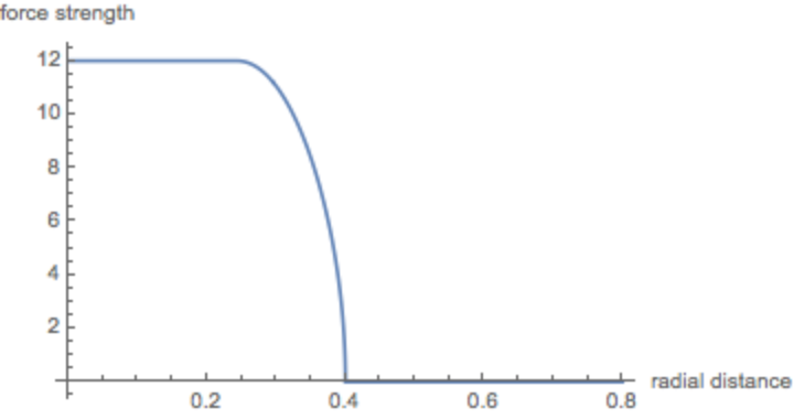
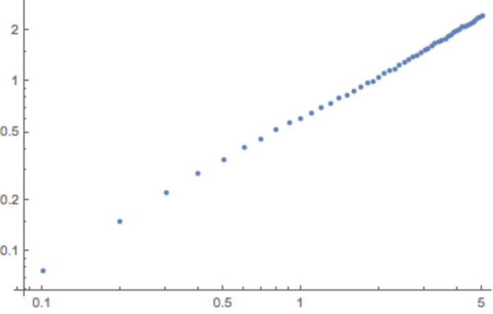
Sketch of the force law of α=1/2 and hardness 12 of a peg:
| In[6]:= |
![board = <|
"RowCount" -> 12, "PegRadius" -> 0.4, "PegHardness" -> 12,
"PegForceExponent" -> 1/2,
"PegRotation" -> 0,
"VerticalAcceleration" -> 1,
"LinearFrictionCoefficient" -> 0.3,
"QuadraticFrictionCoefficient" -> 0.2,
"BallRadius" -> 0.05|>;
ResourceFunction["GaltonBoardModel"][board, "ForceLawSketch"]](https://www.wolframcloud.com/obj/resourcesystem/images/895/895a0403-4399-4c3f-b413-14abc3a23f23/4f59110770b464a0.png)
|
| Out[6]= |
|
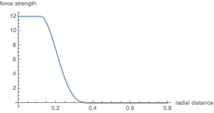
The force law for α=4:
| In[7]:= |
|
| Out[7]= |
|
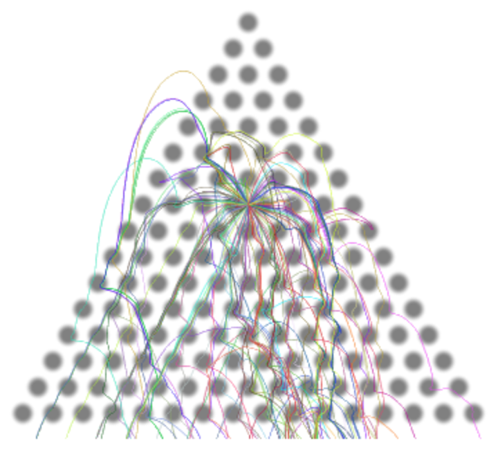
Use nonvanishing initial velocities for the balls (all originating from a single point):
| In[8]:= |
![board = <|
"RowCount" -> 24, "PegRadius" -> 0.32, "PegHardness" -> 400,
"PegForceExponent" -> 1,
"PegRotation" -> 0,
"VerticalAcceleration" -> 1,
"LinearFrictionCoefficient" -> 0.,
"QuadraticFrictionCoefficient" -> 1,
"BallRadius" -> 0.|>;
ResourceFunction["GaltonBoardModel"][board, Table[{{0, 1}, 3 RandomReal[{-1, 1}, 2]}, 120], "PathGraphics"]](https://www.wolframcloud.com/obj/resourcesystem/images/895/895a0403-4399-4c3f-b413-14abc3a23f23/24a2c7d3e353b859.png)
|
| Out[8]= |
|
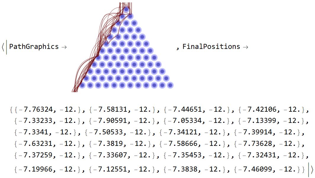
A list of result types returns an association of results:
| In[9]:= |
![board = <|
"RowCount" -> 12, "PegRadius" -> 0.5, "PegHardness" -> 20,
"PegForceExponent" -> 3,
"PegRotation" -> 1.2,
"VerticalAcceleration" -> 1,
"LinearFrictionCoefficient" -> 0.4,
"QuadraticFrictionCoefficient" -> 0.3,
"BallRadius" -> 0.02|>;
ResourceFunction["GaltonBoardModel"][board, Table[{RandomReal[{-1, 1}], 1}, 24],
{"FinalPositions", "PathGraphics"}]](https://www.wolframcloud.com/obj/resourcesystem/images/895/895a0403-4399-4c3f-b413-14abc3a23f23/26dc75ac6957ef84.png)
|
| Out[10]= |
|
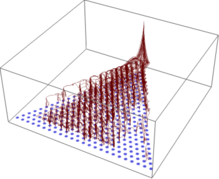
Show the speed of the balls as the vertical function value:
| In[11]:= |
![board = <|
"RowCount" -> 24, "PegRadius" -> 0.32, "PegHardness" -> 40,
"PegForceExponent" -> 1,
"PegRotation" -> 0,
"VerticalAcceleration" -> 1,
"LinearFrictionCoefficient" -> 0.,
"QuadraticFrictionCoefficient" -> 1,
"BallRadius" -> 0.|>;
ResourceFunction["GaltonBoardModel"][board, Table[{{0, 1}, 3 RandomReal[{-1, 1}, 2]}, 60], "PathSpeedGraphics3D"]](https://www.wolframcloud.com/obj/resourcesystem/images/895/895a0403-4399-4c3f-b413-14abc3a23f23/6643745fda06d00c.png)
|
| Out[11]= |
|
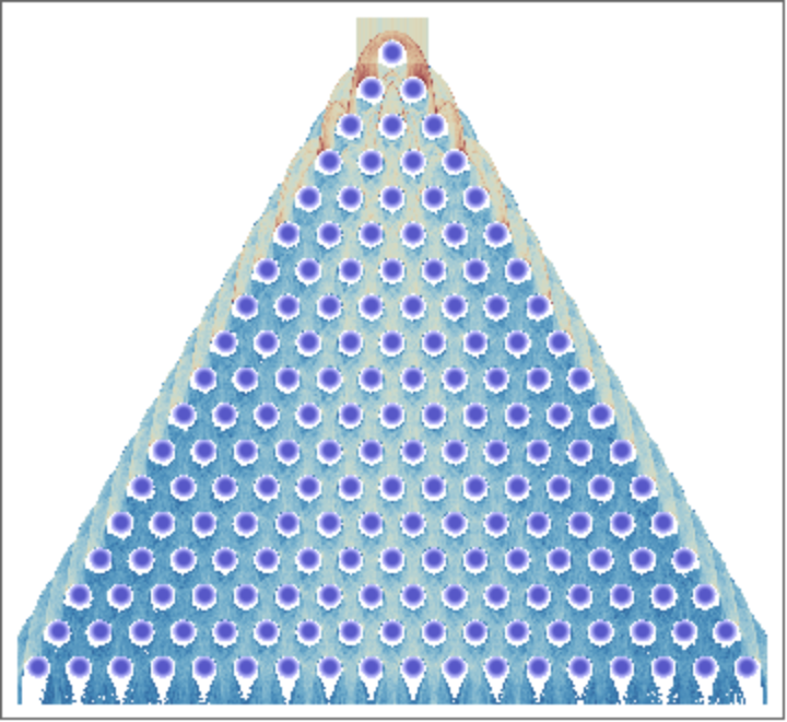
Displaying many (tens of thousands or even hundreds of thousands) of paths would result in large graphics with many ball paths. Returning the result as an array plot is much more memory efficient:
| In[12]:= |
![ResourceFunction["GaltonBoardModel"][<|
"RowCount" -> 18, "PegRadius" -> 0.3, "PegHardness" -> 100,
"PegForceExponent" -> 3/2,
"PegRotation" -> 0,
"VerticalAcceleration" -> 1,
"LinearFrictionCoefficient" -> 0.8,
"QuadraticFrictionCoefficient" -> 0,
"BallRadius" -> 0.1|>, Table[{RandomReal[{-1, 1}], 1}, 100], {"PathArrayPlot", 1200}]](https://www.wolframcloud.com/obj/resourcesystem/images/895/895a0403-4399-4c3f-b413-14abc3a23f23/0a43098333c52771.png)
|
| Out[12]= |
|
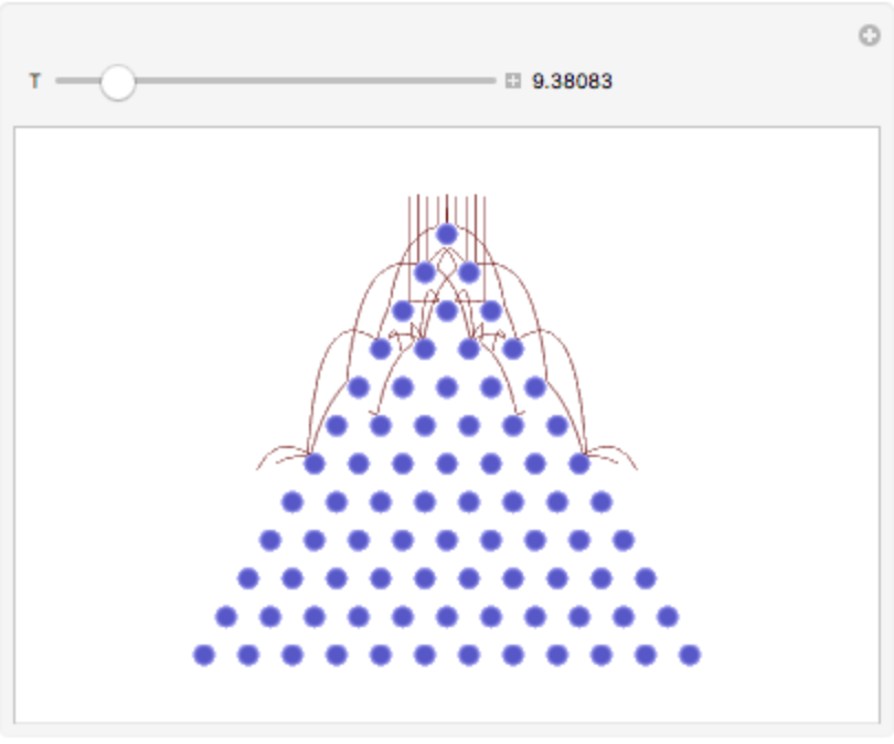
Return an interactive demonstration/animation showing the time-dependent paths of the balls:
| In[13]:= |
![ResourceFunction["GaltonBoardModel"][<|
"RowCount" -> 12, "PegRadius" -> 0.3, "PegHardness" -> 20,
"PegForceExponent" -> 0.8,
"PegRotation" -> 0,
"VerticalAcceleration" -> 1,
"LinearFrictionCoefficient" -> 0.4,
"QuadraticFrictionCoefficient" -> 0.2,
"BallRadius" -> 0.1|>, Table[{x, 1}, {x, -1, 1, 2/8}], "TimeEvolution"]](https://www.wolframcloud.com/obj/resourcesystem/images/895/895a0403-4399-4c3f-b413-14abc3a23f23/0b9ff9e4e8fa0c8a.png)
|
| Out[13]= |
|
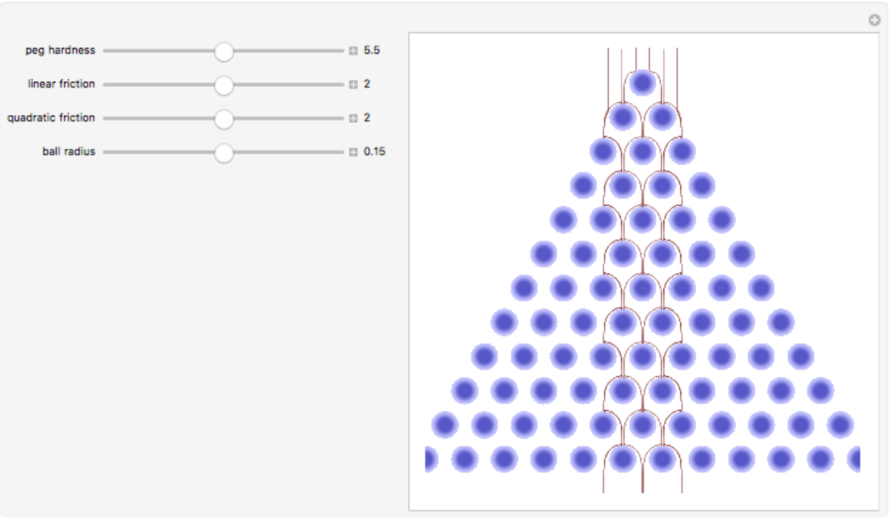
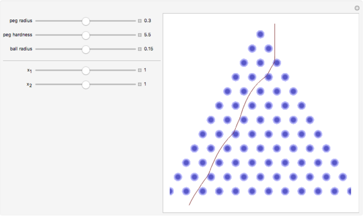
Interactively explore the ball paths as a function of some of the board parameters:
| In[14]:= |
![board = <|
"RowCount" -> 12, "PegRadius" -> 0.4, "PegHardness" -> Interval[{1, 10.}],
"PegForceExponent" -> 2,
"PegRotation" -> 0,
"VerticalAcceleration" -> 1,
"LinearFrictionCoefficient" -> Interval[{0, 4}],
"QuadraticFrictionCoefficient" -> Interval[{0, 4}],
"BallRadius" -> Interval[{0, 0.3}]|>;
ResourceFunction["GaltonBoardModel"][board, Table[{x, 1}, {x, -1, 1, 2/5}], "Manipulate"]](https://www.wolframcloud.com/obj/resourcesystem/images/895/895a0403-4399-4c3f-b413-14abc3a23f23/277c465f969f62f8.png)
|
| Out[14]= |
|
Also include the initial conditions in the interactive controls:
| In[15]:= |
![board = <|
"RowCount" -> 12, "PegRadius" -> Interval[{0, 0.6}], "PegHardness" -> Interval[{1, 10.}],
"PegForceExponent" -> 2,
"PegRotation" -> 0,
"VerticalAcceleration" -> 1,
"LinearFrictionCoefficient" -> 0.2,
"QuadraticFrictionCoefficient" -> 0.2,
"BallRadius" -> Interval[{0, 0.3}]|>;
ResourceFunction[
"GaltonBoardModel"][board, {Interval[{0, 2}], Interval[{0, 2}]}, "Manipulate"]](https://www.wolframcloud.com/obj/resourcesystem/images/895/895a0403-4399-4c3f-b413-14abc3a23f23/377e18a5bdb60e71.png)
|
| Out[15]= |
|
The ball paths in a relatively bouncy set of pegs:
| In[16]:= |
![board = <|
"RowCount" -> 24, "PegRadius" -> 0.25, "PegHardness" -> 80,
"PegForceExponent" -> 2,
"PegRotation" -> 0,
"VerticalAcceleration" -> 1,
"LinearFrictionCoefficient" -> 0.5,
"QuadraticFrictionCoefficient" -> 0.1,
"BallRadius" -> 0.1|>;
ResourceFunction["GaltonBoardModel"][board, Table[{RandomReal[{-1, 1}], 1}, 20], "PathGraphics"]](https://www.wolframcloud.com/obj/resourcesystem/images/895/895a0403-4399-4c3f-b413-14abc3a23f23/0235c01567821ab2.png)
|
| Out[17]= |
|
Compute the arrival (at the imaginary row 25) for 1,000 balls:
| In[18]:= |
|
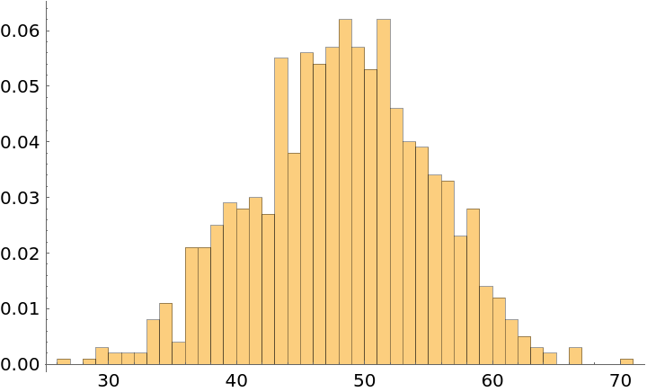
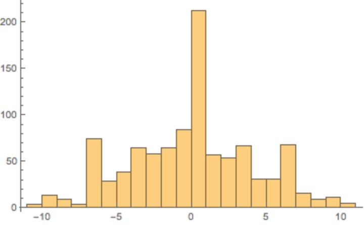
Plot the histogram of the distribution of the arrival times:
| In[19]:= |
|
| Out[19]= |
|
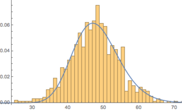
Fit with a typical first-hit distribution for Brownian motion with drift:
| In[20]:= |
![bins = {#1, #2/1000} & @@@ Tally[Round[tAs]];
NonlinearModelFit[bins, a Exp[-(b - c t)^2/(2 t)]/Sqrt[2 Pi t^3], {{a, 50}, {b, 42}, {c, 1}}, t] // Normal](https://www.wolframcloud.com/obj/resourcesystem/images/895/895a0403-4399-4c3f-b413-14abc3a23f23/269092bfba96fbf5.png)
|
| Out[21]= |

|
| In[22]:= |
|
| Out[22]= |
|
In modeling the result for a Galton board with large pegs, many balls never penetrate the interior regions between the pegs:
| In[23]:= |
![board = <|
"RowCount" -> 24, "PegRadius" -> 0.4, "PegHardness" -> 8,
"PegForceExponent" -> 5/2,
"PegRotation" -> 0,
"VerticalAcceleration" -> 1,
"LinearFrictionCoefficient" -> 0,
"QuadraticFrictionCoefficient" -> 2,
"BallRadius" -> 0.02|>;
SeedRandom[1234];
ResourceFunction["GaltonBoardModel"][board, Table[{{0, 1}, 10 Normalize[RandomReal[{-1, 1}, 2]]}, 10], "PathGraphics"]](https://www.wolframcloud.com/obj/resourcesystem/images/895/895a0403-4399-4c3f-b413-14abc3a23f23/6d01e894e6d3b3a1.png)
|
| Out[24]= |
|
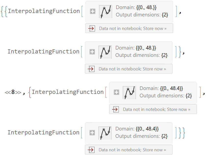
Obtain the interpolating functions for the positions and velocities for 10 paths:
| In[25]:= |
![SeedRandom[1234];
ifs = ResourceFunction["GaltonBoardModel"][board, Table[{{0, 1}, 10 Normalize[RandomReal[{-1, 1}, 2]]}, 10], "InterpolatingFunctions"];
Short[ifs, 2]](https://www.wolframcloud.com/obj/resourcesystem/images/895/895a0403-4399-4c3f-b413-14abc3a23f23/20fcfe12b6830a82.png)
|
| Out[26]= |
|
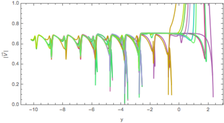
Show the speed versus the vertical coordinate ![]() for all paths:
for all paths:
| In[27]:= |
![yV[t_Real, {ifX_, ifV_}] := {Last[ifX[t]], Norm[ifV[t]]}
ParametricPlot[Evaluate[Style[yV[t, #], RandomColor[]] & /@ ifs],
{t, 0, 20}, AspectRatio -> 1/2, Frame -> True, Axes -> False, FrameLabel -> {"y", "|\!\(\*OverscriptBox[\(V\), \(\[RightVector]\)]\)|"},
PlotRange -> {All, {0, 1}}]](https://www.wolframcloud.com/obj/resourcesystem/images/895/895a0403-4399-4c3f-b413-14abc3a23f23/53c5d011068d8ac2.png)
|
| Out[27]= |
|
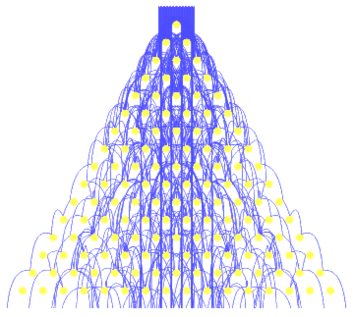
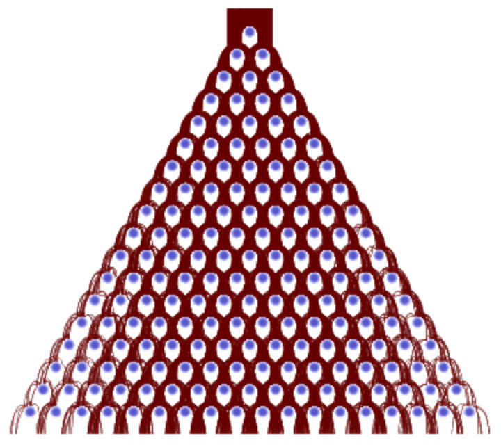
Specify yellow pegs and blue ball paths:
| In[28]:= |
![board = <|
"RowCount" -> 16, "PegRadius" -> 0.25, "PegHardness" -> 100,
"PegRotation" -> 0,
"PegForceExponent" -> 1,
"VerticalAcceleration" -> 1,
"LinearFrictionCoefficient" -> 0.5,
"QuadraticFrictionCoefficient" -> 0.3,
"BallRadius" -> 0.|>;
ResourceFunction["GaltonBoardModel"][board, Table[{x, 1}, {x, -1, 1, 2/120}], "PathGraphics", "TrajectoryStyle" -> Directive[Thickness[0.001], Opacity[0.8], Lighter[Blue, 0.3]],
"PegStyle" -> {Directive[Yellow, Opacity[0.66]], White}]](https://www.wolframcloud.com/obj/resourcesystem/images/895/895a0403-4399-4c3f-b413-14abc3a23f23/075afadd5cf20396.png)
|
| Out[28]= |
|
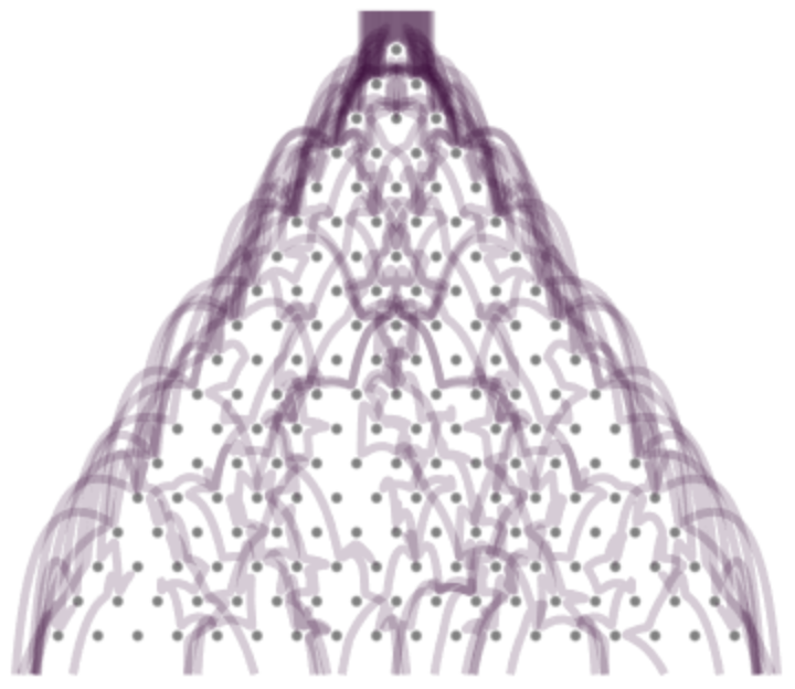
To visualize a finite ball size, specify Thickness[Automatic] in the "TrajectoryStyle" option setting to obtain "thick" ball paths:
| In[29]:= |
![board = <|
"RowCount" -> 18, "PegRadius" -> 0.2, "PegHardness" -> 100,
"PegRotation" -> 0,
"PegForceExponent" -> 3/2,
"VerticalAcceleration" -> 1,
"LinearFrictionCoefficient" -> 0.5,
"QuadraticFrictionCoefficient" -> 0,
"BallRadius" -> 0.2|>;
ResourceFunction["GaltonBoardModel"][board, Table[{x, 1}, {x, -1, 1, 2/36}], "PathGraphics", "PegStyle" -> {Gray, White},
"TrajectoryStyle" -> Directive[Thickness[Automatic], Opacity[0.2], Darker[Purple, 0.6]]]](https://www.wolframcloud.com/obj/resourcesystem/images/895/895a0403-4399-4c3f-b413-14abc3a23f23/5ea5d9e121b469ae.png)
|
| Out[29]= |
|
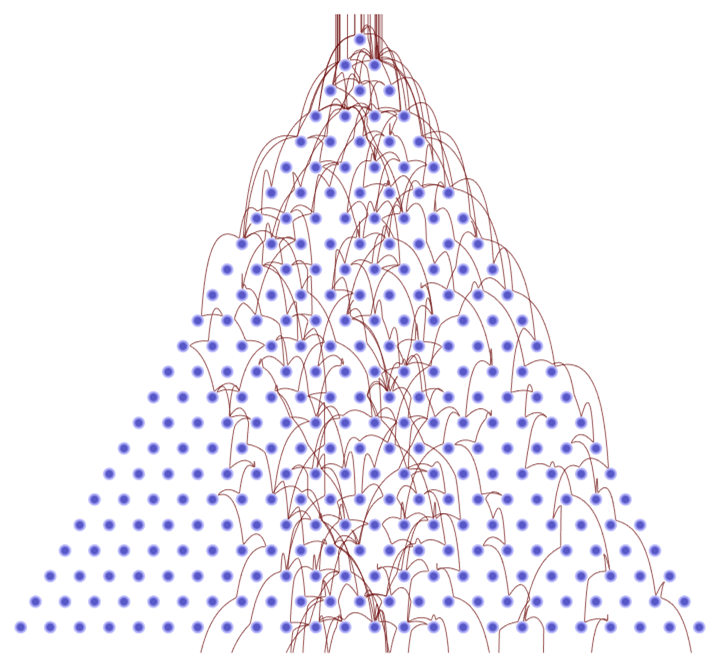
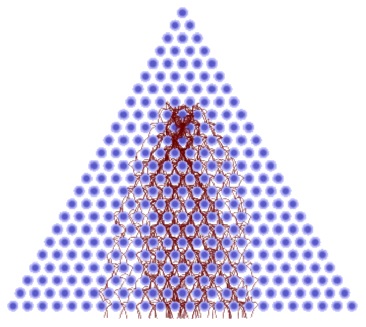
Show regression to the center for a board:
| In[30]:= |
![board = <|
"RowCount" -> 18, "PegRadius" -> 0.25, "PegHardness" -> 40,
"PegForceExponent" -> 3/2,
"PegRotation" -> 0,
"VerticalAcceleration" -> 1,
"LinearFrictionCoefficient" -> 0.4,
"QuadraticFrictionCoefficient" -> 1,
"BallRadius" -> 0.1|>;
{gr, fps} = ResourceFunction["GaltonBoardModel"][board, Table[{RandomReal[{-1, 1}], 1}, 1000],
{"PathGraphics", "FinalPositions"}] // Normal;](https://www.wolframcloud.com/obj/resourcesystem/images/895/895a0403-4399-4c3f-b413-14abc3a23f23/5347eb49270d55f1.png)
|
The balls' paths:
| In[31]:= |
|
| Out[31]= |
|
The final positions of the balls:
| In[32]:= |
|
| Out[32]= |
|
Bin the data under the last row of pegs:
| In[33]:= |
|
Show a histogram of the binned data:
| In[34]:= |
|
| Out[34]= |
|
Fit the final positions to a normal distribution:
| In[35]:= |
|
| Out[35]= |
|
Because of the binning, a direct test fails:
| In[36]:= |
|
| Out[36]= |
|
Use bootstrapping and collect statistics:
| In[37]:= |
![testStatisticSample = Block[{bootstrap, gd},
Table[bootstrap = RandomVariate[estDist, Length[bins]];
gd = Round[bootstrap, Sqrt[3]/2]; DistributionFitTest[gd, estDist, "TestStatistic"], {100}]];](https://www.wolframcloud.com/obj/resourcesystem/images/895/895a0403-4399-4c3f-b413-14abc3a23f23/169eb2ae15e08289.png)
|
Compute the p-value:
| In[38]:= |
|
| Out[38]= |
|
Compute the autocorrelation function ![]() for the ball position.
for the ball position.
Start the balls from deep within the board:
| In[39]:= |
![board = <|
"RowCount" -> 24, "PegRadius" -> 0.45, "PegHardness" -> 100,
"PegForceExponent" -> 5/2,
"PegRotation" -> 0,
"VerticalAcceleration" -> 1,
"LinearFrictionCoefficient" -> 0,
"QuadraticFrictionCoefficient" -> 1,
"BallRadius" -> 0.05|>;
ResourceFunction["GaltonBoardModel"][board, Table[{{0, -9}, 10 Normalize[RandomReal[{-1, 1}, 2]]}, 50], "PathGraphics"]](https://www.wolframcloud.com/obj/resourcesystem/images/895/895a0403-4399-4c3f-b413-14abc3a23f23/15e9d49cb3c8d69c.png)
|
| Out[39]= |
|
Get the interpolating functions of the ball paths:
| In[40]:= |
|
Define the position autocorrelation function by averaging along each path as well as over all paths:
| In[41]:= |
|
| In[42]:= |
|
Plot c(τ) as a function of τ:
| In[43]:= |
|
| Out[43]= |
|
Fit c(τ) to a power law c(τ)~τβ; the value β≲0.5 indicates subdiffusive movement:
| In[44]:= |
|
| Out[44]= |
|
Very small vertical acceleration turns the Galton board into a classical Lorenz gas:
| In[45]:= |
![board = <|
"RowCount" -> 24, "PegRadius" -> 0.4, "PegHardness" -> 12,
"PegForceExponent" -> 0.3,
"PegRotation" -> 0,
"VerticalAcceleration" -> 0.1,
"LinearFrictionCoefficient" -> 0,
"QuadraticFrictionCoefficient" -> 0.2,
"BallRadius" -> 0.1|>;
ResourceFunction["GaltonBoardModel"][board, Table[{{0, -11}, 5 Normalize[RandomReal[{-1, 1}, 2]]}, 5], "PathGraphics", "PegStyle" -> {Gray, White},
"TrajectoryStyle" :> Directive[Opacity[0.6], Thickness[0.002], RandomColor[]]] // Quiet](https://www.wolframcloud.com/obj/resourcesystem/images/895/895a0403-4399-4c3f-b413-14abc3a23f23/22a1b31b5a17adfa.png)
|
| Out[45]= |
|
Negative friction coefficients (modeling autonomous balls) and rotating peg forces (modeling rotating pegs) can lead to unusual path shapes:
| In[46]:= |
![board = <|
"RowCount" -> 16, "PegRadius" -> 0.5, "PegHardness" -> 4,
"PegForceExponent" -> 2,
"PegRotation" -> 1.4,
"VerticalAcceleration" -> 1,
"LinearFrictionCoefficient" -> -2,
"QuadraticFrictionCoefficient" -> 2,
"BallRadius" -> 0.1|>;
ResourceFunction["GaltonBoardModel"][board, Table[{{0, -7}, 5 Normalize[RandomReal[{-1, 1}, 2]]}, 120], "PathGraphics", "PegStyle" -> {Gray, White},
"TrajectoryStyle" :> Directive[Opacity[0.6], Thickness[0.002], RandomColor[]]]](https://www.wolframcloud.com/obj/resourcesystem/images/895/895a0403-4399-4c3f-b413-14abc3a23f23/13efce5d7950a7ed.png)
|
| Out[46]= |
|
Inject balls with slightly different initial conditions to see the trajectories diverge after multiple peg collisions:
| In[47]:= |
|
| In[48]:= |
![ResourceFunction["GaltonBoardModel"][board, Table[{{2 + 0.4 RandomReal[{-1, 1}], 1},
{-5, -4}}, {60}], "PathGraphics",
"TrajectoryStyle" :> Directive[Opacity[0.6], Thickness[0.004], RandomColor[]],
"PegStyle" -> {Directive[Gray, Opacity[0.5]], White}]](https://www.wolframcloud.com/obj/resourcesystem/images/895/895a0403-4399-4c3f-b413-14abc3a23f23/3ac482a3ce2082f6.png)
|
| Out[48]= |
|
Retrieve some "random" boards with preselected parameters:
| In[49]:= |
|
| Out[49]= |

|
| In[50]:= |
|
| Out[50]= |

|
| In[51]:= |
|
| Out[51]= |
|
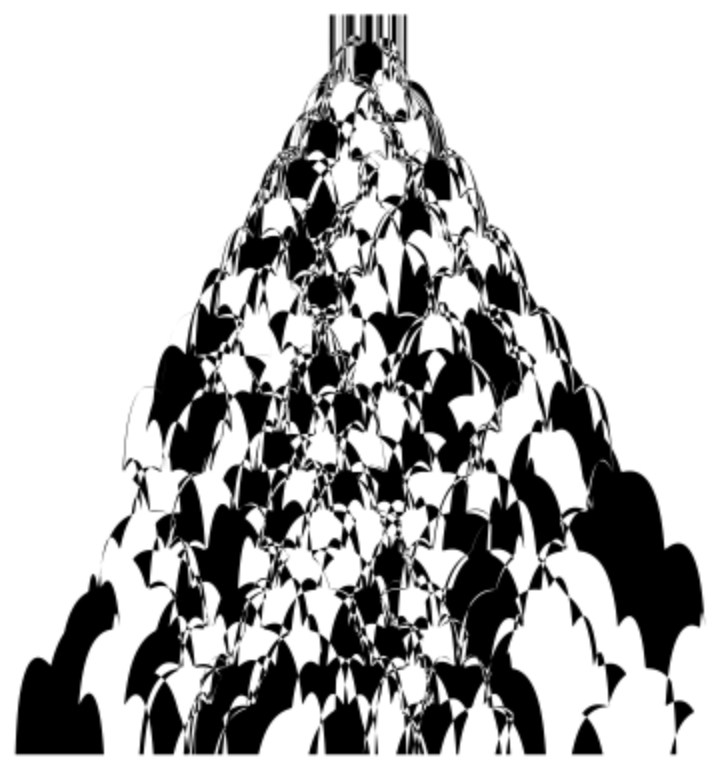
Connect ball trajectories and form an intricate polygon:
| In[52]:= |
|
| In[53]:= |
|
| In[54]:= |
![Show[Graphics[
Polygon[Join @@ MapIndexed[If[OddQ[#2[[1]]], #1, Reverse[#1]] &, First /@ Cases[paths, _Line, \[Infinity]]]]]]](https://www.wolframcloud.com/obj/resourcesystem/images/895/895a0403-4399-4c3f-b413-14abc3a23f23/257185932b3fb9da.png)
|
| Out[54]= |
|
This work is licensed under a Creative Commons Attribution 4.0 International License