Wolfram Function Repository
Instant-use add-on functions for the Wolfram Language
Function Repository Resource:
Get a point belonging to the Faure sequence
ResourceFunction["FaurePoint"][k,d,b] gives the kth d-dimensional point belonging to the base-b Faure sequence. | |
ResourceFunction["FaurePoint"][k,d] automatically chooses the base. |
A 2D Faure point:
| In[1]:= |
| Out[1]= |
A 3D Faure point:
| In[2]:= |
| Out[2]= |
Use a different base:
| In[3]:= |
| Out[3]= |
FaurePoint threads elementwise over lists:
| In[4]:= |
| Out[4]= |
Show the structure of a Faure sequence in dimension 2:
| In[5]:= |
| Out[5]= | 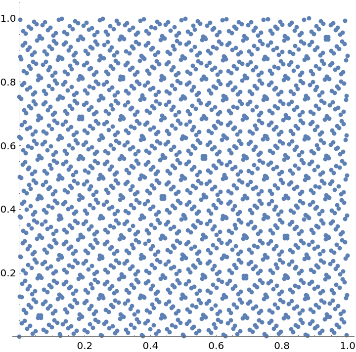 |
Use the Faure sequence to approximate π by quasi-Monte Carlo integration:
| In[6]:= |
| Out[6]= |
Use RescalingTransform to map Faure sequence points to other rectangular or cuboidal domains:
| In[7]:= | ![Graphics3D[
Sphere[RescalingTransform[
ConstantArray[{0, 1}, 3], {{1, 3}, {-1, 1}, {0, 2}}][
ResourceFunction["FaurePoint"][Range[0, 3^7 - 1], 3]], 0.02]]](https://www.wolframcloud.com/obj/resourcesystem/images/7ea/7ea2b207-b9ef-4853-8e3f-f2b512d0ba60/2d453bc50597ec2d.png) |
| Out[7]= | 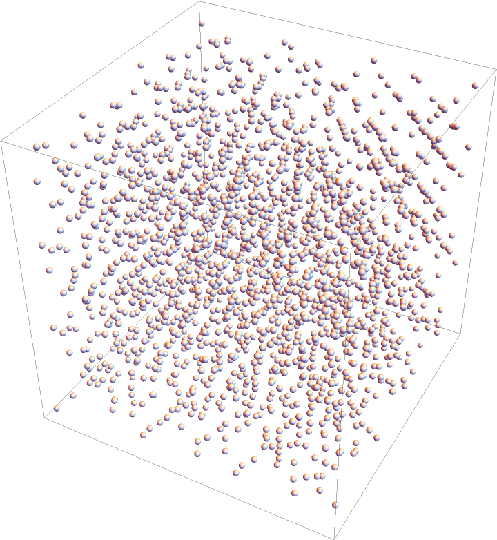 |
If the unit square is divided into rectangles with area b-n, each rectangle contains exactly one member of the first bn points generated by the base b Faure sequence:
| In[8]:= | ![With[{b = 2, n = 8, p = 4, q = 4},
ListPlot[ResourceFunction["FaurePoint"][Range[0, b^n - 1], 2, b], AspectRatio -> 1, GridLines -> {Subdivide[b^p], Subdivide[b^q]}, GridLinesStyle -> Directive[AbsoluteThickness[2]], PlotRange -> {{0, 1}, {0, 1}}, PlotStyle -> AbsolutePointSize[2]]]](https://www.wolframcloud.com/obj/resourcesystem/images/7ea/7ea2b207-b9ef-4853-8e3f-f2b512d0ba60/167ad9eefc4a77a5.png) |
| Out[8]= | 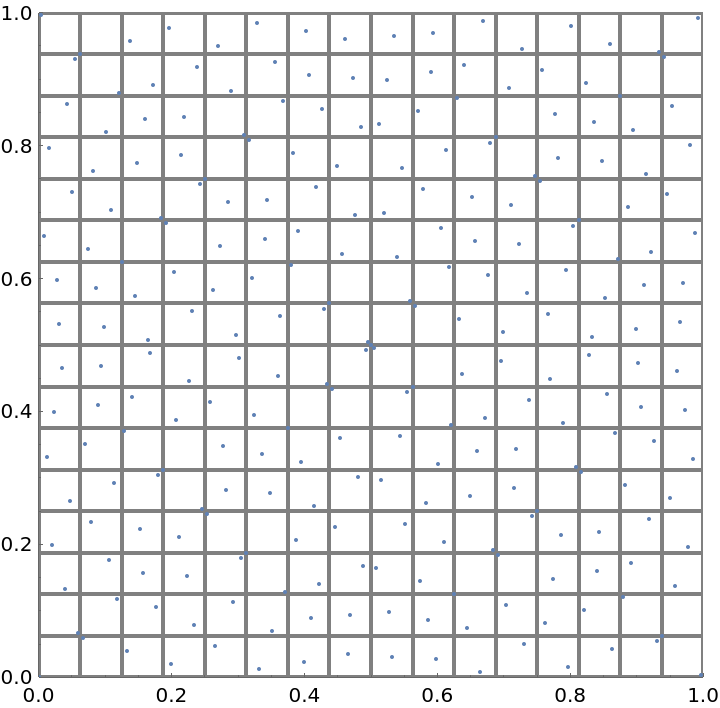 |
This work is licensed under a Creative Commons Attribution 4.0 International License