Wolfram Function Repository
Instant-use add-on functions for the Wolfram Language
Function Repository Resource:
Display an L-system
ResourceFunction["LSystemPlot"][rules,axiom,n,delta] displays the L-string for the nth iteration of the list rules, starting with the string axiom after n iterations with an angle delta. |
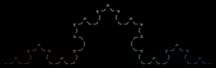
Four steps for Koch quadratic rules:
| In[1]:= |
|
| Out[1]= |
|
Get just the resulting string after only one step:
| In[2]:= |
|
| Out[2]= |
|
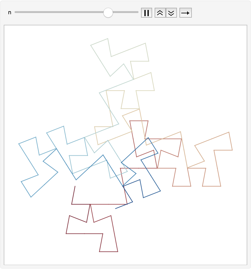
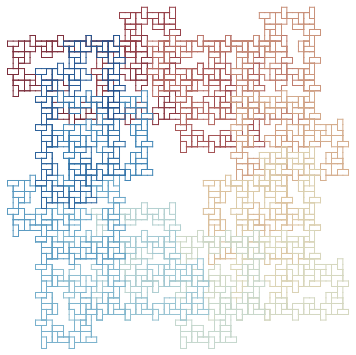
Continuously modify the angle:
| In[3]:= |
![Animate[ResourceFunction[
"LSystemPlot"][{"F" -> "-F+F-F-F+F+FF-F+F+FF+F-F-FF+FF-FF+F+F-FF-F-F+FF-F-F+F+F-F+"}, "F+F+F+F", 1, n Degree, ColorFunction -> ColorData["RedBlueTones"]], {n, 30., 120.}]](https://www.wolframcloud.com/obj/resourcesystem/images/7d8/7d8df8c4-be7b-41c9-a957-b0e9c2dde206/69b2f2f493e72a82.png)
|
| Out[3]= |
|
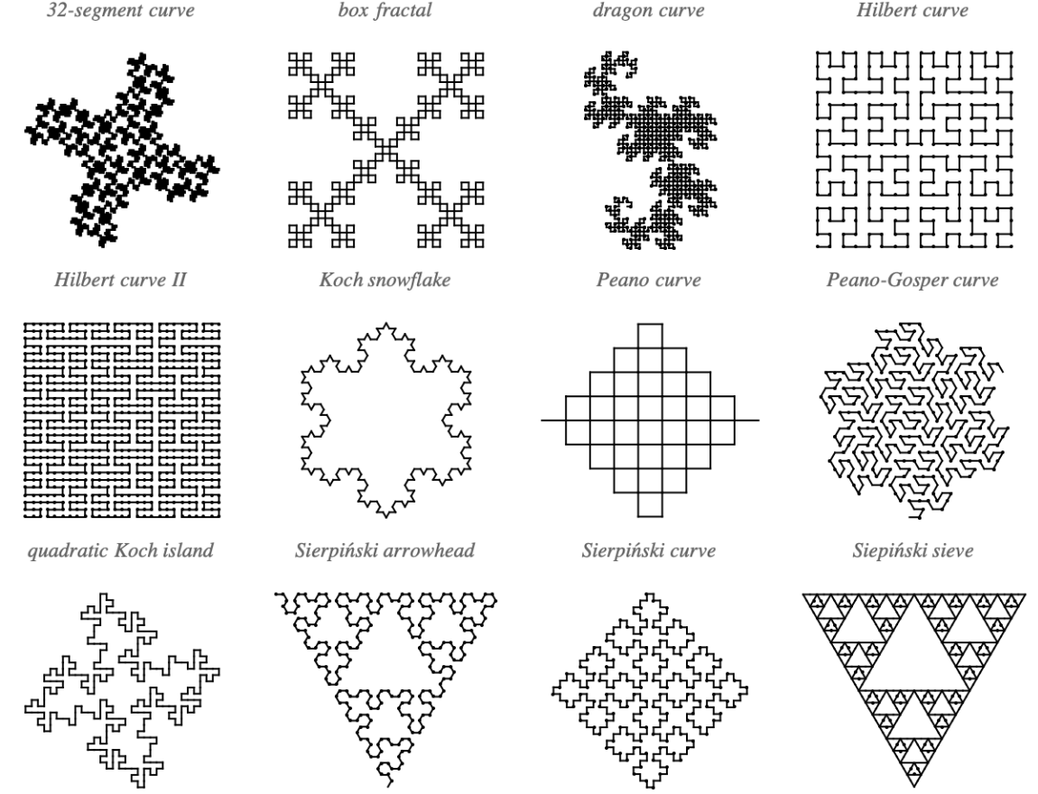
Grid for named fractals:
| In[4]:= |
![lsystems = {{"32\[Hyphen]segment curve", {"F" -> "-F+F-F-F+F+FF-F+F+FF+F-F-FF+FF-FF+F+F-FF-F-F+FF-F-F+F+F-F+"}, "F+F+F+F", 2, 90},
{"box fractal", {"F" -> "F-F+F+F-F"}, "F-F-F-F", 3, 90}, {"dragon curve", {"X" -> "X+YF+", "Y" -> "-FX-Y"}, "FX", 10, 90}, {"Hilbert curve", {"L" -> "+RF-LFL-FR+", "R" -> "-LF+RFR+FL-"}, "L", 4, 90}, {"Hilbert curve II", {"X" -> "XFYFX+F+YFXFY-F-XFYFX", "Y" -> "YFXFY-F-XFYFX+F+YFXFY"}, "X", 3, 90},
{"Koch snowflake", {"F" -> "F+F--F+F"}, "F--F--F", 3, 60}, {"Peano curve", {"F" -> "F+F-F-F-F+F+F+F-F"}, "F", 2, 90}, {"Peano\[Hyphen]Gosper curve", {"X" -> "X+YF++YF-FX--FXFX-YF+", "Y" -> "-FX+YFYF++YF+FX--FX-Y"}, "FX", 3, 60}, {"quadratic Koch island", {"F" -> "F-F+F+FFF-F-F+F"}, "F+F+F+F", 2, 90}, {"Sierpiński arrowhead", {"X" -> "YF+XF+Y", "Y" -> "XF-YF-X"}, "YF", 5, 60}, {"Sierpiński curve", {"X" -> "XF-F+F-XF+F+XF-F+F-X"}, "F+XF+F+XF", 3, 90}, {"Siepiński sieve", {"F" -> "FF", "X" -> "--FXF++FXF++FXF--"}, "FXF--FF--FF", 4, 60}};](https://www.wolframcloud.com/obj/resourcesystem/images/7d8/7d8df8c4-be7b-41c9-a957-b0e9c2dde206/78f7a48b980dcf9c.png)
|
| In[5]:= |
![GraphicsGrid[
Partition[
ResourceFunction["LSystemPlot"][Sequence @@ (Take[#, {2, -2}]), Last[#] Degree // N, PlotLabel -> First[#], BaseStyle -> {FontFamily -> "Times", FontSlant -> "Italic"}] & /@
lsystems,
4], ImageSize -> 600]](https://www.wolframcloud.com/obj/resourcesystem/images/7d8/7d8df8c4-be7b-41c9-a957-b0e9c2dde206/57828b3e96013eaf.png)
|
| Out[5]= |
|
Select a gradient color function:
| In[6]:= |
|
| Out[6]= |
|
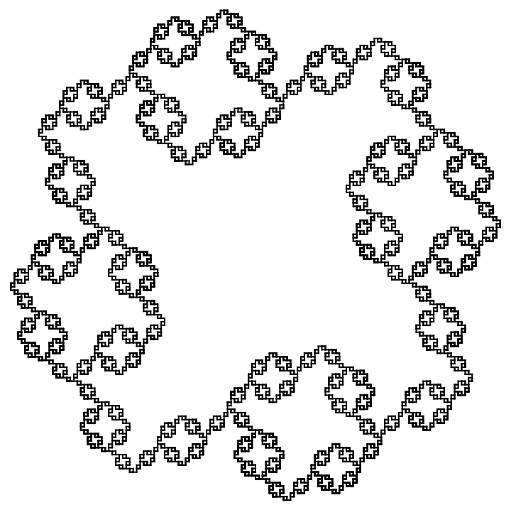
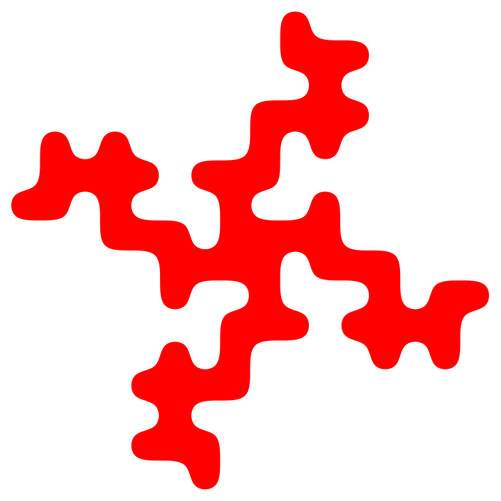
Convert to a BSplineCurve:
| In[8]:= |
![sc32 = ResourceFunction[
"LSystemPlot"][{"F" -> "-F+F-F-F+F+FF-F+F+FF+F-F-FF+FF-FF+F+F-FF-F-F+FF-F-F+F+F-F+"}, "F+F+F+F", 1];](https://www.wolframcloud.com/obj/resourcesystem/images/7d8/7d8df8c4-be7b-41c9-a957-b0e9c2dde206/4878eb8fa68edc1f.png)
|
| In[9]:= |
|
| Out[9]= |
|
| In[10]:= |
|
| Out[10]= |
|
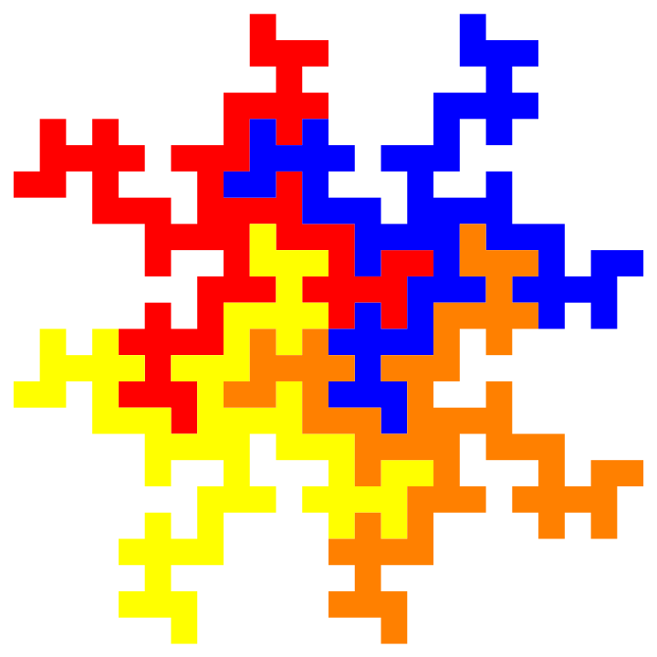
Make a tessellation:
| In[11]:= |
![With[{fc = Polygon[Cases[sc32, Line[{a_, b_}] -> a, \[Infinity]]]}, Graphics[{Red, fc, Blue, Translate[fc, {8, 0}], Yellow, Translate[fc, {0, -8}], Orange, Translate[fc, {8, -8}]}]]](https://www.wolframcloud.com/obj/resourcesystem/images/7d8/7d8df8c4-be7b-41c9-a957-b0e9c2dde206/5f246065442db701.png)
|
| Out[11]= |
|
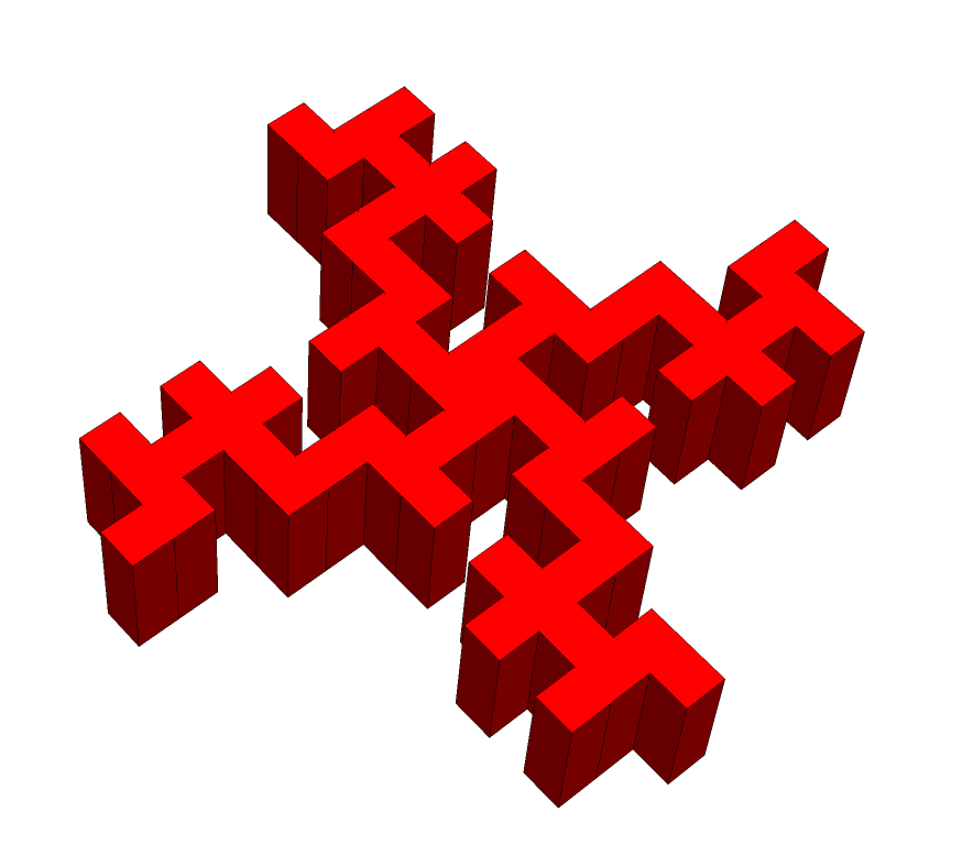
Go to 3D:
| In[12]:= |
![coords = With[{pts = Cases[sc32, Line[{a_, b_}] -> a, \[Infinity]]}, {(Polygon[{Append[#1[[1]], 0.], Append[#1[[2]], 0.], Append[#1[[2]], 3.], Append[#1[[1]], 3.]}] &) /@ Partition[pts, 2, 1], Polygon[Append[#1, 3.] & /@ pts]}];](https://www.wolframcloud.com/obj/resourcesystem/images/7d8/7d8df8c4-be7b-41c9-a957-b0e9c2dde206/0058f557e53dffab.png)
|
| In[13]:= |
|
| Out[13]= |
|
Wolfram Language 11.3 (March 2018) or above
This work is licensed under a Creative Commons Attribution 4.0 International License