Basic Examples (6)
The data below is monotonic, and we get a monotonic interpolation:
Plot the function:
Next we see the function fun perfectly interpolates the data:
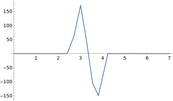
The following suggests the derivative of fun is positive over the interval {0,7}:
The derivative of fun is well behaved:
The second derivative of fun is continuous:
Scope (3)
MonotonicInterpolation can handle exact data provided all values are real numbers:
The InterpolatingFunction above only gives MachinePrecision results:
f[1] evaluates to a MachinePrecision approximation of 4-ⅇ:
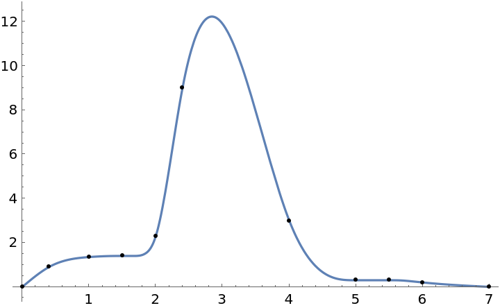
The next data has a local maximum at {2.4,9} and the InterpolatingFunction will have a local max someplace between x = 2 and x = 4. MonotonicInterpolation tries to find the smoothest InterpolatingFunction with no local min and no other local max; more precisely, MonotonicInterpolation tries to minimize 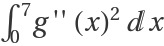 with only one extremum:
The following suggests g' is positive for all values in the interval {0,2.84} and never positive for values in the interval {2.841,7}:
Two adjacent data samples above are {5,0.3}, {5.5,0.3}. Since these samples have equal y-values, g' is zero at all x in the interval {5,5.5}:
Using the same data, but unsorted, results in the same InterpolatingFunction:
Options (11)
KnotsBetweenSamples (3)
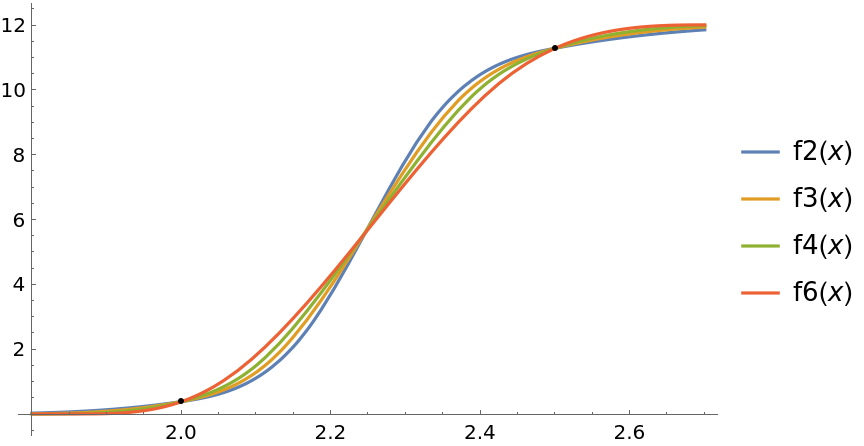
More knots between each pair of samples will give smoother interpolations:
The derivative of the InterpolatingFunction changes more slowly as the setting of the KnotsBetweenSamples option is increased:
The integral of the second derivative squared decreases as the setting of "KnotsBetweenSamples" is increased:
MaxIterations (4)
MonotonicInterpolation passes the setting of MaxIterations directly to QuadraticOptimization:
Below a low setting for MaxIterations allows a solution to be found in less time than the default setting, but the quality of the solution may be sacrificed:
Integrating of the second derivative squared shows that default is smoother than f10. This is explained by the message above:
There is a slight difference between the InterpolatingFunction objects found above:
Tolerance (4)
The default setting has the Tolerance determined automatically, but it is not able to find an InterpolatingFunction in this next example:
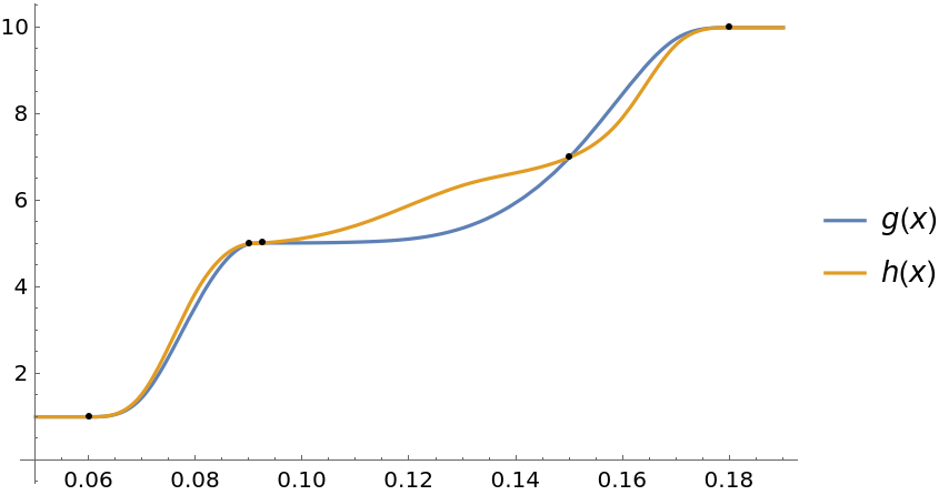
Two monotonic interpolating functions of the data above are found using specific settings for Tolerance:
We see there are significant differences between the above interpolating functions:
Integrating of the second derivative squared shows that g is smoother than h:
Applications (4)
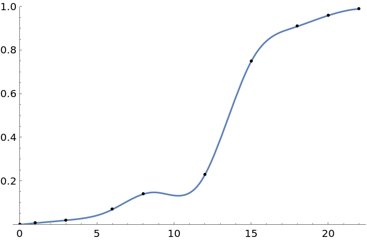
Given data representing the fraction of a population of dogs that died at or before a certain age, we use Interpolation to create a continuous function describing the fraction of dogs that that would have died by any age less than 22:
The next cell indicates that 13.25% of dogs would die at or before 10.25 years age, while the data provided says 14.0% of dogs died at or before 8 years of age. These are not compatible, so the above is not a very good InterpolatingFunction for this application:
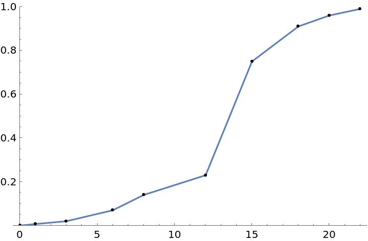
The previous example requires a monotonically increasing InterpolatingFunction. Using the data above, we could have met that requirement if we used Interpolation[data,Method→"Hermite"], but that is not guaranteed to give a monotonic InterpolatingFunction for every monotonic set of data. Instead we can use linear interpolation as in the next cell, and that is guaranteed to give a monotonic InterpolatingFunction for every monotonic set of data:
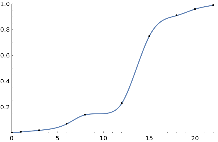
However, this linear interpolation doesn’t have a continuous first derivative. It is reasonable to expect that the actual curve is smooth, and MonotonicInterpolation below tries to find the smoothest possible monotonically-increasing InterpolatingFunction that interpolates the monotonic data. The interpolation shown below is monotonic over the whole range plotted and it’s first two derivatives are continuous:
Properties and Relations (8)
Below, MonotonicInterpolation returns an expression with the built-in head InterpolatingFunction:
We can use any of the following methods on an InterpolatingFunction:
Next we get a lists of the x-values and y-values used to define the InterpolatingFunction fun:
The InterpolatingFunction fun also has specified derivatives at each of the x-values. Those derivatives can be retrieved from the internal representation of the InterpolatingFunction shown below:
Get the derivative of the fun[x] at corresponding x-values:
Get an expression used in the definition of the InterpolatingFunction fun:
Next we see how the above expression was used to define the InterpolatingFunction fun:
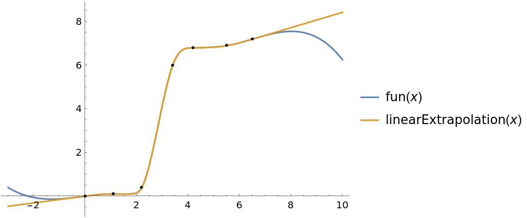
The InterpolatingFunction fun is effectively a different cubic polynomial over several intervals. If we evaluate fun[x] using an x outside the domain of fun, it uses the cubic polynomial form the nearest end of the domain. The next cell performs surgery on the above expression to make an new InterpolatingFunction that extends the domain of the original function using linear extrapolation:
Possible Issues (2)
MonotonicInterpolation will often fail to find an InterpolatingFunction when some samples are very close together as in this example:
The number of unknowns that QuadraticOptimization needs to determine is Length[data]+2(Length[data]-1)*"KnotsBetweenSamples", and the time required for QuadraticOptimization to find a solution is proportional to (number of unknowns)3. As a result, the time MonotonicInterpolation requires increases dramatically as the setting for "KnotsBetweenSamples" increases. Also, when the setting for "KnotsBetweenSamples" is too large, the limitations of MachinePrecision arithmetic often prevent QuadraticOptimization from finding a solution. An example of that is given in the next cell that takes a few minutes to evaluate:
Neat Examples (1)
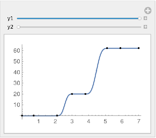
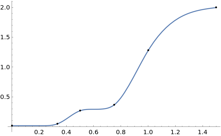
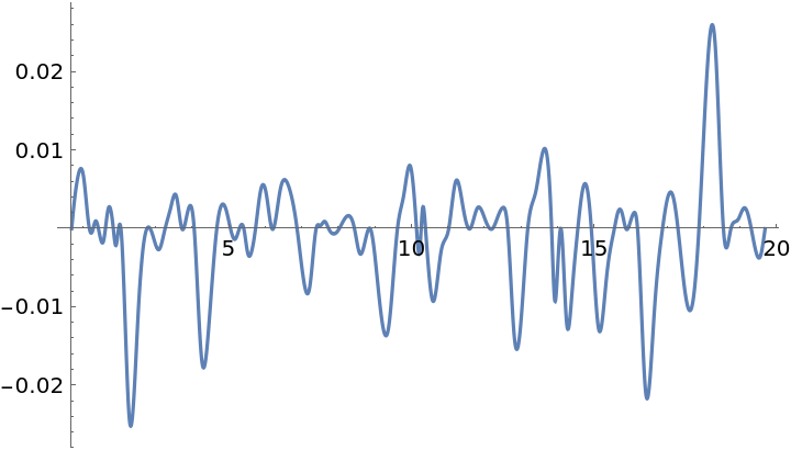
MonotonicInterpolation is efficient enough to use in Manipulate when the List of data is not too long:
![data = {{0, E^-4}, {1/3, E^-3}, {1/2, 1/(1 + E)}, {3/4, 1/E}, {1, 4 - E}, {3/2, 2}};
f = ResourceFunction["MonotonicInterpolation"][data];
Plot[f[x], {x, 0, 3/2}, Epilog -> Point@data, PlotRange -> All]](https://www.wolframcloud.com/obj/resourcesystem/images/7c4/7c455180-f390-4cea-a081-37d3b4482c6e/32353c36fe53fd1c.png)
![data = {{0, 0}, {0.4, 0.9}, {1, 1.35}, {1.5, 1.4}, {2, 2.3}, {2.4, 9}, {4, 3}, {5, 0.3}, {5.5, 0.3}, {6, 0.2}, {7, 0.0}};
g = ResourceFunction["MonotonicInterpolation"][data];
Plot[g[x], {x, 0, 7}, Epilog -> Point@data, PlotRange -> All]](https://www.wolframcloud.com/obj/resourcesystem/images/7c4/7c455180-f390-4cea-a081-37d3b4482c6e/0d957c33156ebdc1.png)

![data = {{1.5, 1.4}, {0.4, 0.9}, {7, 0.0}, {1, 1.35}, {0, 0}, {2, 2.3}, {5.5, 0.3}, {2.4, 9}, {4, 3}, {6, 0.2}, {5, 0.3}};
h = ResourceFunction["MonotonicInterpolation"][data];
Plot[h[x], {x, 0, 7}, Epilog -> Point@data, PlotRange -> All]](https://www.wolframcloud.com/obj/resourcesystem/images/7c4/7c455180-f390-4cea-a081-37d3b4482c6e/50e47c514a67ba0f.png)
![(* Evaluate this cell to get the example input *) CloudGet["https://www.wolframcloud.com/obj/8c4e5251-e3e0-4216-a7cf-5fdba1143a2d"]](https://www.wolframcloud.com/obj/resourcesystem/images/7c4/7c455180-f390-4cea-a081-37d3b4482c6e/603bdd6b27dfb134.png)
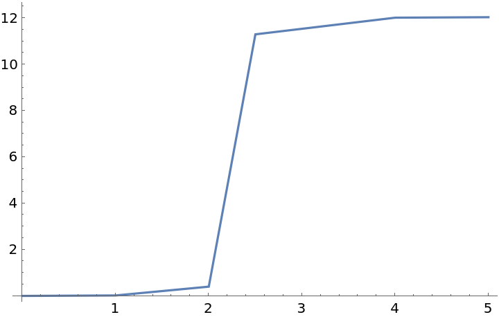
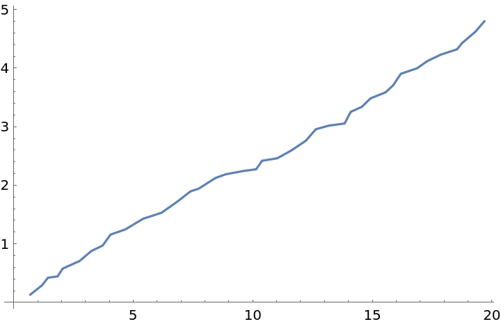
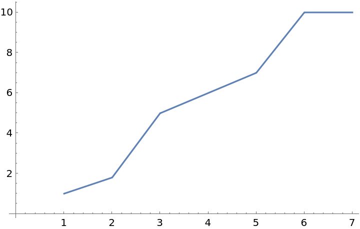
![SeedRandom[1234];
xs = Accumulate@RandomReal[{0.2, 0.75}, 40];
ys = Accumulate@RandomReal[{0.02, 0.2}, 40];
data = Transpose@{xs, ys};
ListLinePlot[data]](https://www.wolframcloud.com/obj/resourcesystem/images/7c4/7c455180-f390-4cea-a081-37d3b4482c6e/317221c675d65723.png)
![data = {{0, 0}, {1, 0.007}, {3, 0.02}, {6, 0.07}, {8, 0.14}, {12, 0.23}, {15, 0.75}, {18, 0.91}, {20, 0.96}, {22, 0.99}};
fractionDied = Interpolation[data, Method -> "Spline", InterpolationOrder -> 3];
Plot[fractionDied[years], {years, 0, 22}, PlotRange -> {0, 1}, Epilog -> Point@data]](https://www.wolframcloud.com/obj/resourcesystem/images/7c4/7c455180-f390-4cea-a081-37d3b4482c6e/16a8f112ed148052.png)


![{{x1}, y1, yp1} = Part[expression, 1];
{{xn}, yn, ypn} = Part[expression, -1];
expression = Join[{{{-10000}, y1 + yp1 (x1 - 10000), yp1}}, expression, {{{10000}, yn + ypn (10000 - xn), ypn}}];
linearExtrapolation = Interpolation[expression];
Plot[{fun[x], linearExtrapolation[x]}, {x, -3, 10}, Epilog -> Point@data, PlotLegends -> "Expressions"]](https://www.wolframcloud.com/obj/resourcesystem/images/7c4/7c455180-f390-4cea-a081-37d3b4482c6e/68417bf3526ef8ca.png)
![Manipulate[
data = {{0, 0.0}, {0.7, 0.02}, {2.1, 0.06}, {3, y1}, {3.8, y2}, {5.1,
62.2}, {5.9, 62.24}, {7, 62.26}};
fun = Quiet@ResourceFunction["MonotonicInterpolation"][data];
Plot[fun[x], {x, 0, 7}, Epilog -> Point@data],
{{y1, 20}, 0.06, 20}, {{y2, 20}, 20, 62.2}]](https://www.wolframcloud.com/obj/resourcesystem/images/7c4/7c455180-f390-4cea-a081-37d3b4482c6e/137b86ac9bb364ac.png)