Wolfram Function Repository
Instant-use add-on functions for the Wolfram Language
Function Repository Resource:
Find the best-fit sphere for a set of points
ResourceFunction["SphereFit"][pts] returns the best-fit Sphere for the points pts. | |
ResourceFunction["SphereFit"][w→pts] returns the best-fit Sphere using the weights w. | |
ResourceFunction["SphereFit"][pts,"Association"] returns an Association with the center, radius, Sphere, and a pure function defining the sphere. |
Find the best-fit Sphere for the given points:
| In[1]:= |
| Out[2]= |
See the result along with the points:
| In[3]:= |
| Out[5]= | 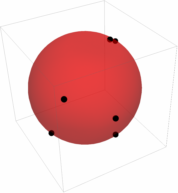 |
Fit a sphere through a noisy 1000 points:
| In[6]:= | ![pts = Normalize /@ RandomVariate[NormalDistribution[], {1000, 3}];
pts *= RandomVariate[NormalDistribution[5, 0.25], Length[pts]];
pts += Threaded[{100, 200, 300}];
Graphics3D[{Black, Sphere[pts, 0.1], Red, Opacity[0.5], ResourceFunction["SphereFit"][pts]}]](https://www.wolframcloud.com/obj/resourcesystem/images/749/74929467-489e-4d6c-8aa7-195a2c44efb4/1f8b74ebb2a30e02.png) |
| Out[9]= |  |
Get all the properties:
| In[10]:= |
| Out[11]= |  |
Use the "Function" to create a definition of the sphere:
| In[12]:= |
| Out[12]= |
Specify weights for outliers:
| In[13]:= | ![pts = {{-1, -1, -1}, {-1, -1, 1}, {-1, 1, -1}, {-1, 1, 1}, {1, -1, -1}, {1, -1, 1}, {1, 1, -1}, {1, 1, 3}};
weights = {1, 1, 1, 1, 1, 1, 1, 0.1};
Graphics3D[{Black, Sphere[pts, 0.2], Red, Opacity[0.5], ResourceFunction["SphereFit"][weights -> pts]}]](https://www.wolframcloud.com/obj/resourcesystem/images/749/74929467-489e-4d6c-8aa7-195a2c44efb4/439cd584c327203c.png) |
| Out[15]= | 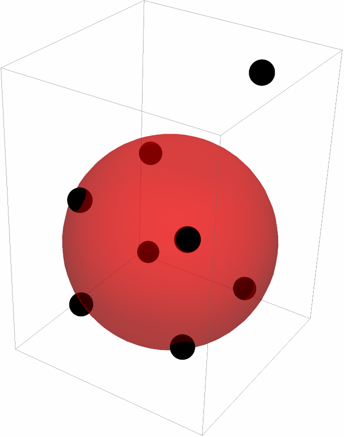 |
For two points, the fit goes through both:
| In[16]:= | ![pts = {{2, -1, -1}, {-1, -2, 3}};
Graphics3D[{Black, Sphere[pts, 0.2], Red, Opacity[0.5], ResourceFunction["SphereFit"][pts]}]](https://www.wolframcloud.com/obj/resourcesystem/images/749/74929467-489e-4d6c-8aa7-195a2c44efb4/6209b5a561b14e00.png) |
| Out[17]= | 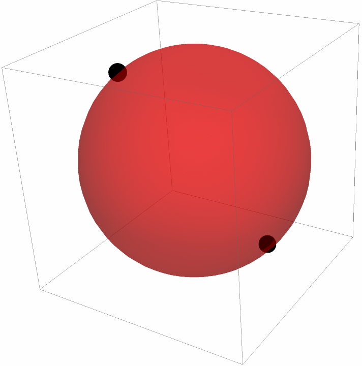 |
For three points, the fit goes through all the points:
| In[18]:= | ![pts = {{2, -1, -1}, {-1, -2, 3}, {2, 3, 6}};
Graphics3D[{Black, Sphere[pts, 0.2], Red, Opacity[0.5], ResourceFunction["SphereFit"][pts]}]](https://www.wolframcloud.com/obj/resourcesystem/images/749/74929467-489e-4d6c-8aa7-195a2c44efb4/2228641a0cda1e58.png) |
| Out[19]= | 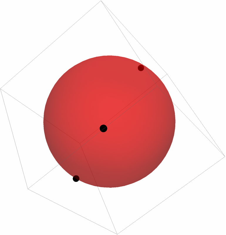 |
For four points, the fit goes through all the points:
| In[20]:= | ![pts = {{2, -1, -1}, {-1, -2, 3}, {2, 4, 3}, {-1, -3, -2}};
Graphics3D[{Black, Sphere[pts, 0.2], Red, Opacity[0.5], ResourceFunction["SphereFit"][pts]}]](https://www.wolframcloud.com/obj/resourcesystem/images/749/74929467-489e-4d6c-8aa7-195a2c44efb4/7d93ecaa7fa06f28.png) |
| Out[21]= | 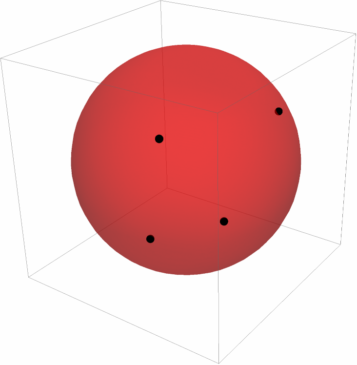 |
If the points fall on a sphere and cover more than a hemisphere, BoundingRegion can give similar results:
| In[22]:= | ![pts = Normalize /@ RandomVariate[NormalDistribution[], {1000, 3}];
pts += Threaded[{100, 200, 300}];
{ResourceFunction["SphereFit"][pts], BoundingRegion[pts, "MinBall"]}](https://www.wolframcloud.com/obj/resourcesystem/images/749/74929467-489e-4d6c-8aa7-195a2c44efb4/59678de807aaac1c.png) |
| Out[24]= |
When 3 points are given and they are collinear, a Failure object is returned:
| In[25]:= |
| Out[25]= |
When 4 or more points are given and they are coplanar, a Failure object is returned:
| In[26]:= | ![SeedRandom[1234];
pts = Table[{0, -1, 3} + t {2, 3, 4}, {t, RandomVariate[NormalDistribution[], 5]}];
ResourceFunction["SphereFit"][pts]](https://www.wolframcloud.com/obj/resourcesystem/images/749/74929467-489e-4d6c-8aa7-195a2c44efb4/6a7324182798468b.png) |
| Out[27]= |
Fit points that only lay on one-eighth of a sphere:
| In[28]:= | ![pts = Normalize /@ RandomVariate[NormalDistribution[], {10000, 3}];
pts //= Select[#[[1]] > 0 \[And] #[[2]] > 0 \[And] #[[3]] > 0 &];
pts *= RandomVariate[NormalDistribution[1, 0.05], Length[pts]];
pts += Threaded[{100, 200, 300}];
Graphics3D[{pts // Point, Opacity[0.5], Red, ResourceFunction["SphereFit"][pts]}]](https://www.wolframcloud.com/obj/resourcesystem/images/749/74929467-489e-4d6c-8aa7-195a2c44efb4/6e395d82383eccc6.png) |
| Out[29]= | 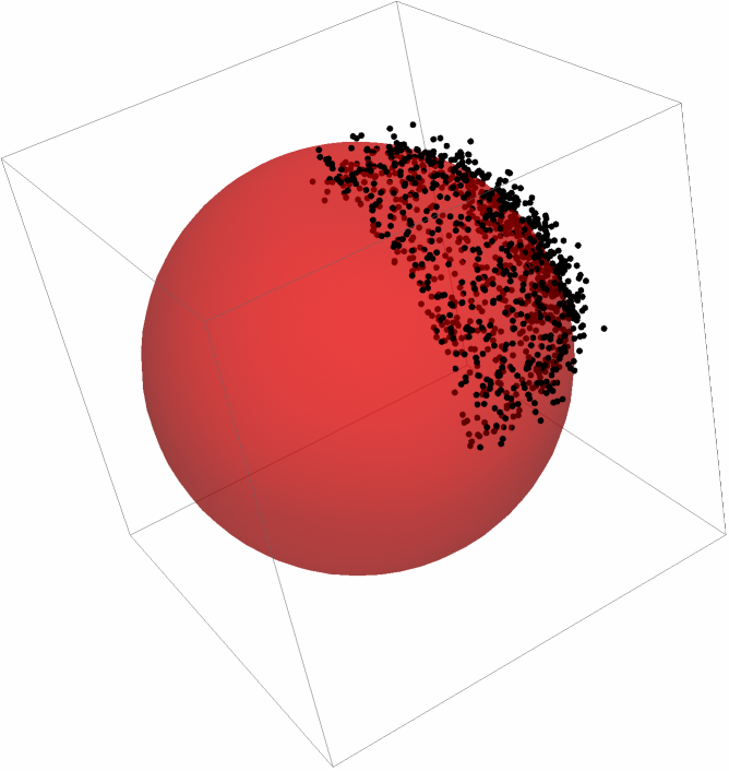 |
Wolfram Language 14.0 (January 2024) or above
First an estimate is found by minimizing ![]() . After that the real problem is minimized using the estimate as a starting points,
. After that the real problem is minimized using the estimate as a starting points, ![]() .
.
This work is licensed under a Creative Commons Attribution 4.0 International License