Wolfram Function Repository
Instant-use add-on functions for the Wolfram Language
Function Repository Resource:
Evaluate the Eisenstein series
ResourceFunction["EisensteinE"][n,q] gives the Eisenstein series En(q). |
Evaluate numerically:
| In[1]:= |
| Out[1]= |
Plot E8(q) over a subset of the reals:
| In[2]:= |
| Out[2]= | 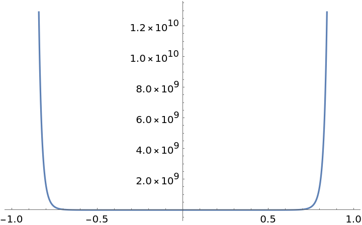 |
Series expansion at the origin:
| In[3]:= |
| Out[3]= |
Evaluate for complex arguments:
| In[4]:= |
| Out[4]= |
Evaluate to high precision:
| In[5]:= |
| Out[5]= |
EisensteinE threads elementwise over lists:
| In[6]:= |
| Out[6]= |  |
Simple exact values are generated automatically:
| In[7]:= |
| Out[7]= |
Plot near the unit circle in the complex q-plane:
| In[8]:= |
| Out[8]= | 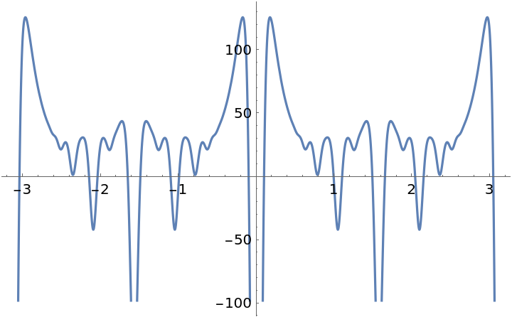 |
| In[9]:= |
| Out[9]= | 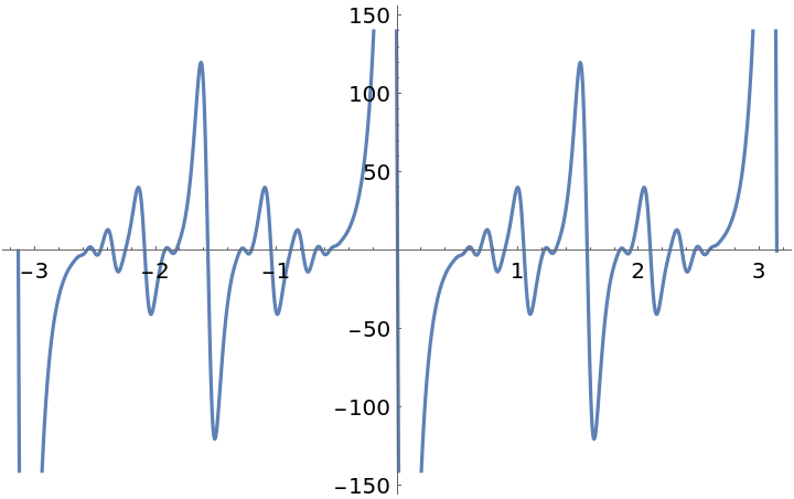 |
EisensteinE[n,q] for n>2 can be expressed in terms of EllipticTheta:
| In[10]:= |
| Out[10]= |  |
WeierstrassInvariants can be expressed in terms of EisensteinE[4,q] and EisensteinE[6,q]:
| In[11]:= |
| Out[12]= |
| In[13]:= |
| Out[13]= |
EisensteinE[n,q] is only defined for positive even n:
| In[14]:= |
| Out[14]= |
Visualize a function with a boundary of analyticity:
| In[15]:= | ![With[{r = 0.995},
ContourPlot[
Arg[ResourceFunction["EisensteinE"][2, qx + I qy]], {qx, -1, 1}, {qy, -1, 1}, {ColorFunction -> (Hue[
Mod[#/(2 Pi), 1]]& ), ColorFunctionScaling -> False, Contours -> 60, ContourLines -> False, Frame -> False, MaxRecursion -> 1, PlotPoints -> 30, PlotRange -> All, RegionFunction -> (Norm[{#, #2}] < r& )}]]](https://www.wolframcloud.com/obj/resourcesystem/images/70b/70bb7854-338c-4a05-aaa5-b304153f4047/5d88e00d4dc6ae0a.png) |
| Out[15]= | 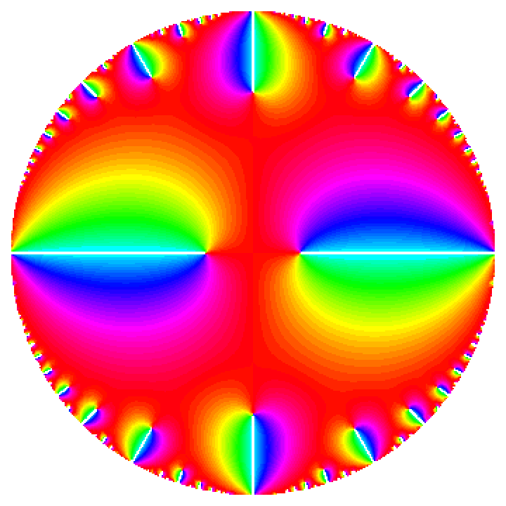 |
| In[16]:= | ![ParametricPlot3D[{qr Cos[q\[Phi]], qr Sin[q\[Phi]], Abs[ResourceFunction["EisensteinE"][2, qr Exp[I q\[Phi]]]]}, {q\[Phi], -\[Pi], \[Pi]}, {qr, 0, 0.99}, BoxRatios -> {1, 1, 0.66}]](https://www.wolframcloud.com/obj/resourcesystem/images/70b/70bb7854-338c-4a05-aaa5-b304153f4047/0d2396d020325d3a.png) |
| Out[16]= | 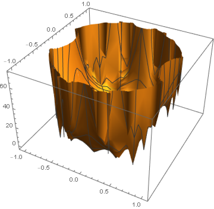 |
This work is licensed under a Creative Commons Attribution 4.0 International License