Basic Examples (2) 

Calculate the confidence level at one standard deviation:

In[1]:=

Out[1]=

Calculate the p-value associated with 3σ:

In[2]:=

Out[2]=

Scope (5) 

SigmaConfidenceLevel returns exact outputs for exact inputs:

In[3]:=

Out[3]=

SigmaConfidenceLevel automatically threads over lists:

In[4]:=

Out[4]=

In physics, a discovery typically has to pass a five-σ of certainty test. Calculate the probability that a five-σ result is not a statistical fluctuation:

In[5]:=

Out[5]=

A p<0.05 test corresponds to a maximum displacement from mean of about 1.64 standard deviations:

In[6]:=

Out[6]=

SigmaConfidenceLevel can be defined as the integral between -σ and σ of the NormalDistribution with mean 0 and standard deviation 1:

In[7]:=

Out[7]=

Applications (1) 

Fit the mean prediction bands of a linear model fit with a confidence level of 1σ, 2σ and 3σ:

In[8]:=

Out[10]=

Properties and Relations (1) 

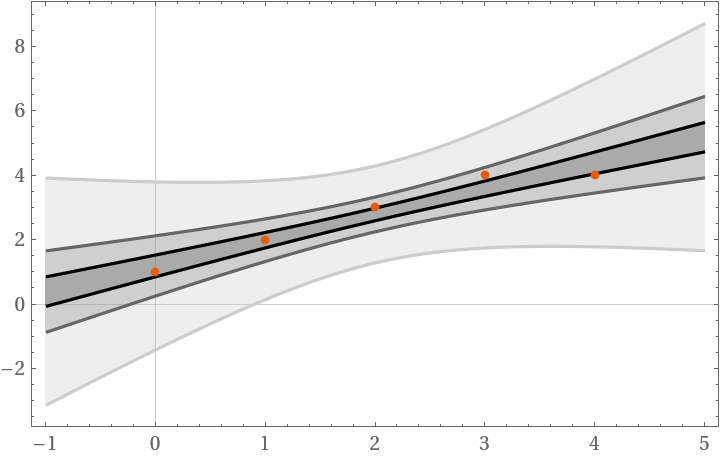SigmaConfidenceLevel handles infinities:

In[11]:=

Out[11]=

Neat Examples (1) 

The 5σ classification limit in physics for discoveries has a false-positive probability of approximately:

In[12]:=

Out[12]=