Wolfram Function Repository
Instant-use add-on functions for the Wolfram Language
Function Repository Resource:
Get an approximation to a parametric curve
ResourceFunction["ApproximatedCurve"][c,{t,t0,tf,n}] computes a line of n points approximating the parametric curve c with t from t0 to tf. | |
ResourceFunction["ApproximatedCurve"][c,{t,t0,tf,n},"type"] gives a result based on "type". |
Approximate cycles around a figure-eight curve:
| In[1]:= |
| Out[1]= |  |
Approximate the curve with lines:
| In[2]:= |
| Out[2]= |  |
Show the lines:
| In[3]:= |
| Out[3]= |  |
Follow a path with arrows:
| In[4]:= |
| Out[4]= |  |
Define a curve in three dimensions:
| In[5]:= |
| Out[5]= |
Polygonal approximation to a curve:
| In[6]:= | ![Show[ParametricPlot3D[helix, {t, 0, 10}], Graphics3D[
ResourceFunction["ApproximatedCurve"][helix, {t, 0, 10, 10}, "Line"]]]](https://www.wolframcloud.com/obj/resourcesystem/images/6f7/6f76840e-ca49-453f-b718-9ebcaeb2881b/3bb687ba5f3e3701.png) |
| Out[6]= | 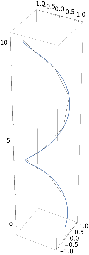 |
Different approximation to a curve:
| In[7]:= |
| Out[7]= | 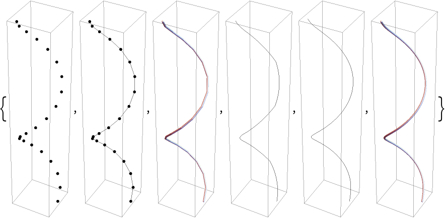 |
Convert points in the following closed curve into a tube. It requires less file space than a full parametrization plot:
| In[8]:= | ![x[t_] := Cos[3 t]
y[t_] := Cos[4 t + Sqrt[2]]
z[t_] := Cos[5 t + Sqrt[3]]](https://www.wolframcloud.com/obj/resourcesystem/images/6f7/6f76840e-ca49-453f-b718-9ebcaeb2881b/7bd729ec42a23bea.png) |
| In[9]:= | ![Graphics3D[
Tube[ResourceFunction[
"ApproximatedCurve"][{x[t], y[t], z[t]}, {t, 0, 10, 15}, BSplineCurve[#, SplineClosed -> True] &], .025]]](https://www.wolframcloud.com/obj/resourcesystem/images/6f7/6f76840e-ca49-453f-b718-9ebcaeb2881b/5e19ba418514e59b.png) |
| Out[9]= | 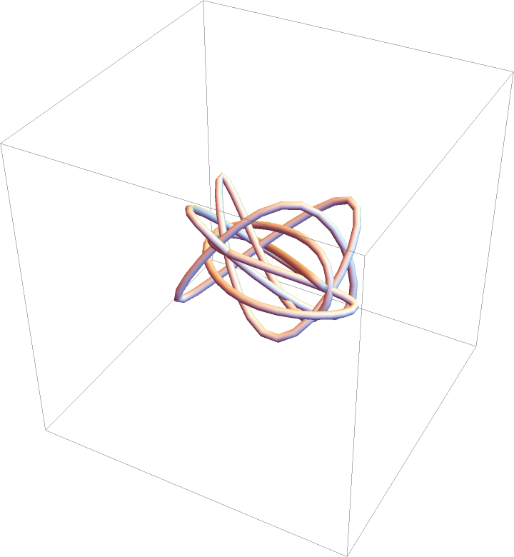 |
Get a curve similar to a handwritten curve:
| In[10]:= |
| Out[10]= |  |
Using AnglePath gives a different curve:
| In[11]:= | ![Graphics[
BSplineCurve[
AnglePath[
ResourceFunction[
"ApproximatedCurve"][{Sin[t], Sin[t] Cos[t]}, {t, 0, 10, 200}, Identity]]]]](https://www.wolframcloud.com/obj/resourcesystem/images/6f7/6f76840e-ca49-453f-b718-9ebcaeb2881b/4f6cc2138cad8877.png) |
| Out[11]= |  |
Define an epicycloid:
| In[12]:= |
| Out[12]= |
Modify it using Accumulate:
| In[13]:= | ![GraphicsRow[{ParametricPlot[Evaluate[ec], {t, 0, 7 \[Pi]}], Graphics[
Line[Accumulate[
N[ResourceFunction["ApproximatedCurve"][ec, {t, 0, 8 \[Pi], 200},
"Coordinates"]]]]]}]](https://www.wolframcloud.com/obj/resourcesystem/images/6f7/6f76840e-ca49-453f-b718-9ebcaeb2881b/6d38a1e54f305a5f.png) |
| Out[13]= |  |
Make a spline from the points of a curve:
| In[14]:= | ![Graphics[
FilledCurve@
ResourceFunction[
"ApproximatedCurve"][{Sin[t], Sin[t] Cos[t]}, {t, 0, 20, 10}, BSplineCurve[#, SplineClosed -> True] &]]](https://www.wolframcloud.com/obj/resourcesystem/images/6f7/6f76840e-ca49-453f-b718-9ebcaeb2881b/283001ee4ca68a4e.png) |
| Out[14]= |  |
Make a design from an epicycloid:
| In[15]:= |
| Out[15]= |
| In[16]:= | ![Show[Graphics[{ResourceFunction["ApproximatedCurve"][
ec, {t, 0, 4 Pi, 20}, "Polygon"]}], ParametricPlot[Evaluate[ec], {t, 0, 4 \[Pi]}]]](https://www.wolframcloud.com/obj/resourcesystem/images/6f7/6f76840e-ca49-453f-b718-9ebcaeb2881b/1ef313aae3ea4910.png) |
| Out[16]= | 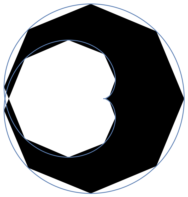 |
Define an epicycloid:
| In[17]:= |
| Out[17]= |
Get a region:
| In[18]:= |
| Out[18]= |
Test if it is a region:
| In[19]:= |
| Out[19]= |
Discretize the region:
| In[20]:= |
| Out[20]= |  |
Compute some properties:
| In[21]:= |
| Out[21]= |
Create and visualize a nephroid:
| In[22]:= | ![Graphics[
Table[Scale[{ColorData["DarkBands"][.025 n], ResourceFunction["ApproximatedCurve"][
Entity["PlaneCurve", "Nephroid"]["ParametricEquations"][1][
t], {t, 0, 2 \[Pi], 12}, "FilledCurve"]}, Log[n]^(-1/2)], {n, 2,
32}]]](https://www.wolframcloud.com/obj/resourcesystem/images/6f7/6f76840e-ca49-453f-b718-9ebcaeb2881b/3341925beea65b82.png) |
| Out[22]= | 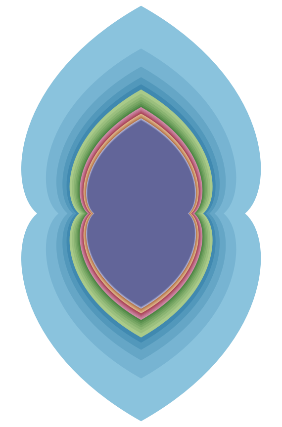 |
A crude approximation to arc length:
| In[23]:= |
| Out[23]= |
| In[24]:= |
| Out[24]= |
Successive approximation to arc length versus the number of steps:
| In[25]:= | ![ListPlot[
Table[Plus @@ ResourceFunction[
"ApproximatedCurve"][{Sin[t], Sin[t] Cos[t]}, {t, 0, 2 \[Pi], n}, EuclideanDistance @@@ Partition[N@#, 2, 1] &], {n, 2, 20}]]](https://www.wolframcloud.com/obj/resourcesystem/images/6f7/6f76840e-ca49-453f-b718-9ebcaeb2881b/66789b1a9a1a0aaf.png) |
| Out[25]= | 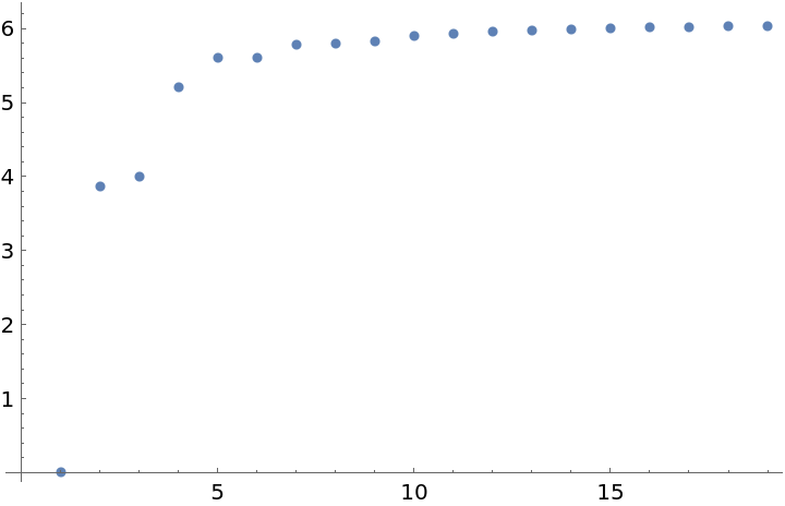 |
Forced undersampling with MaxRecursion and PlotPoints:
| In[26]:= |
| Out[26]= | 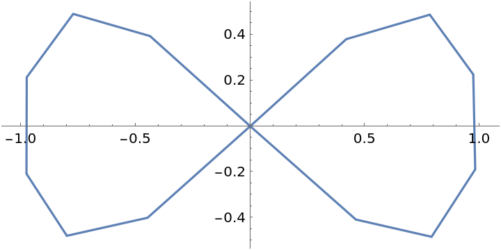 |
Create a similar result using ApproximatedCurve:
| In[27]:= |
| Out[27]= |  |
A polygon gives a similar result to FilledCurve:
| In[28]:= |
| Out[28]= |  |
Generalize CirclePoints:
| In[29]:= |
| In[30]:= | ![Show[Graphics[
ResourceFunction["ApproximatedCurve"][
ellipse[2, 1, t], {t, 0, 2 \[Pi], 10}, "Line"]], ParametricPlot[Evaluate[ellipse[2, 1, t]], {t, 0, 2 \[Pi]}]]](https://www.wolframcloud.com/obj/resourcesystem/images/6f7/6f76840e-ca49-453f-b718-9ebcaeb2881b/0824a4ff24af1241.png) |
| Out[30]= | 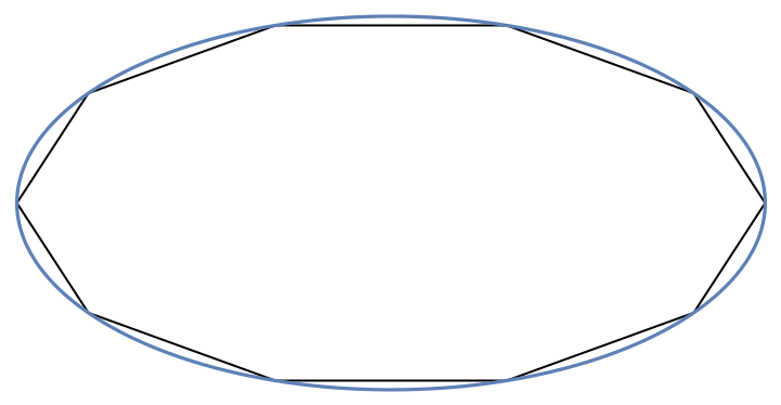 |
Distances between successive points are different:
| In[31]:= |
| Out[31]= |
Show the curve using points:
| In[32]:= | ![Graphics[
Table[{PointSize[.05 n], Hue[1/n], ResourceFunction["ApproximatedCurve"][
ellipse[2, 1, t], {t, 0, 2 \[Pi], 20}, "Point"]}, {n, 5, 1, -1}]]](https://www.wolframcloud.com/obj/resourcesystem/images/6f7/6f76840e-ca49-453f-b718-9ebcaeb2881b/740504e522b8d890.png) |
| Out[32]= | 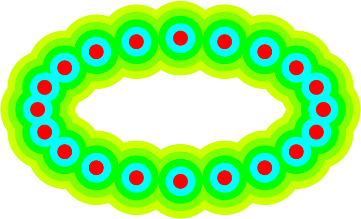 |
Approximate a nephroid:
| In[33]:= |
| Out[33]= |
| In[34]:= | ![Show[Graphics@
ResourceFunction["ApproximatedCurve"][nephroid, {t, 0, 2 \[Pi], 10},
"Line"], ParametricPlot[Evaluate[nephroid], {t, 0, 2 \[Pi]}]]](https://www.wolframcloud.com/obj/resourcesystem/images/6f7/6f76840e-ca49-453f-b718-9ebcaeb2881b/61a8a84691bd7a9d.png) |
| Out[34]= | 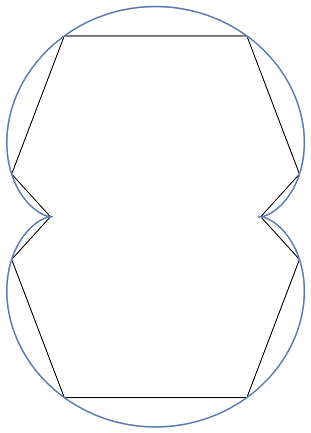 |
This work is licensed under a Creative Commons Attribution 4.0 International License