Basic Examples (2)
The expression of this example has a known symbolic Laplace inverse:
We can compare the result with the answer from the symbolic evaluation:
This expression cannot be inverted symbolically, only numerically:
Scope (2)
The t can be small or large and can contain constants (like π):
Compare with the answer from symbolic evaluation:
The expression Log(p)p is not a Laplace transform of anything because a Laplace transform must tend to zero at p→∞. Nevertheless, numerical inversion returns a result that makes sense:
One way to look at expr4 is  . Note that
  is the Laplace transform of f(t)=-EulerGamma-Log[t], and 0.01 is the second derivative of f(t) at t=10:
In other words, numerical inversion works on a larger class of functions than inversion, but the extension is coherent with the operational rules.
Options (3)
The two options "Startm" and "Method" are introduced here. Consider the following Laplace transform pair:
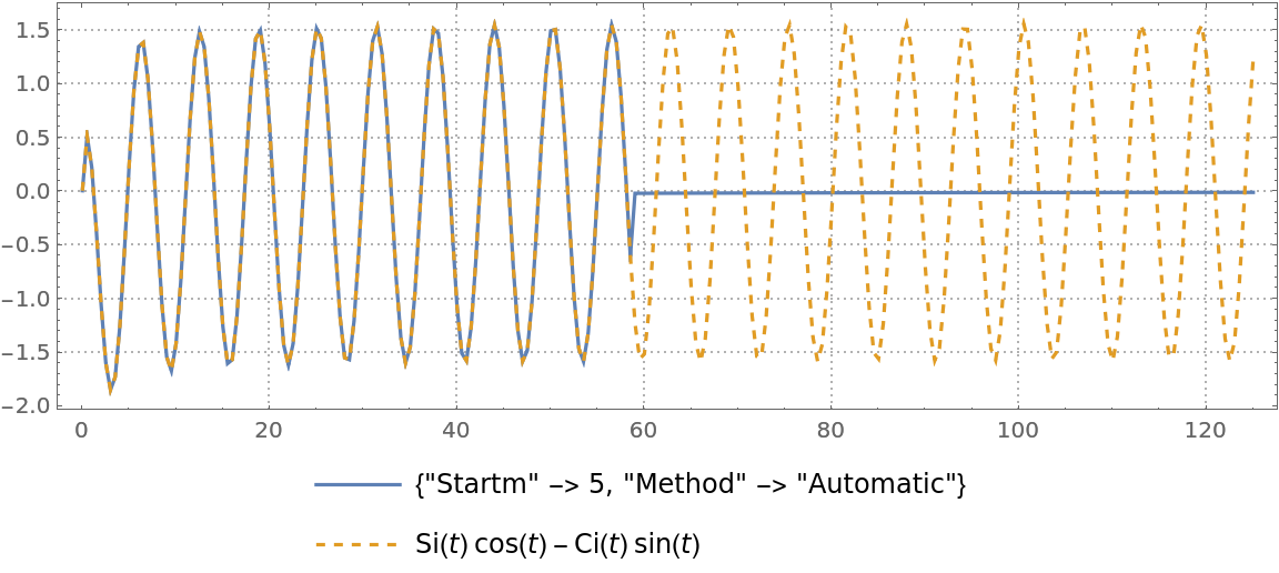
The inverse f5(t) is periodic-like but not exactly periodic. At reasonably small t-values, there is no problem:
But already at the moderate value t=100. we get a surprise:
The result from the NInverseLaplaceTransform function is wrong, and—what is even worse—we do not get an error message. This is what is happening the background: the internal numerical inversion procedures "GWR" (Gaver-Wynn-rho) and "FT" (Fixed-Talbot) provide the same wrong answer initially, so NInverseLaplaceTransform accepts it.
Tackling the problem with the option "Startm"
The default value of the option "Startm" is 5. In the "FT" and "GWR" internal inversion procedures, 2m terms are used, so the default means that initially the number of terms is set to 25=32. For the given problem, this does not provide enough resolution.
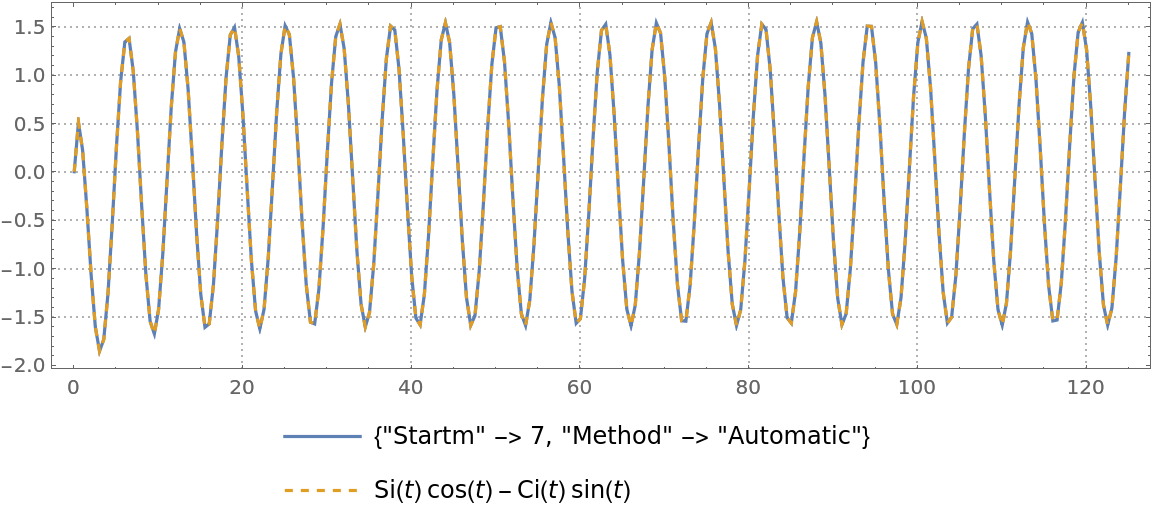
We can try a larger "Startm":
The result is still wrong, but increasing the starting m again provides the correct answer:
Any larger "Startm" would do the same. Changing the default to "Startm"→7—or a larger number—would be, however, a waste of computational resources in most of the cases, so we stick with the default, "Startm"→5 .
Tackling the problem with the option "Method" (1)
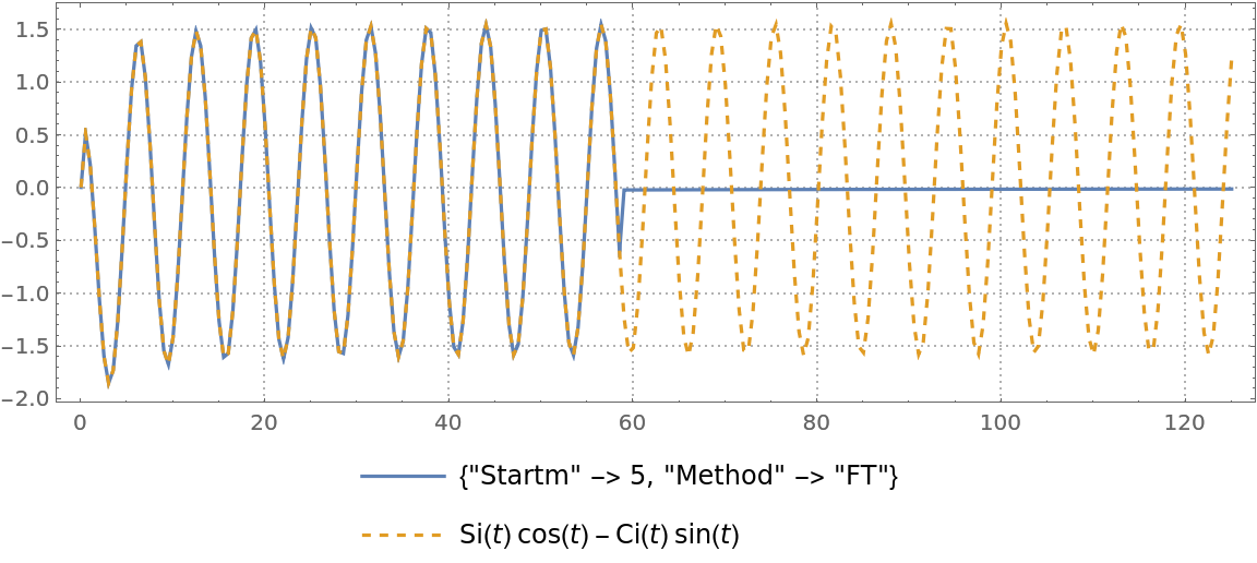
The other option is "Method". It can be "FT", "GWR" or Automatic. The default is Automatic, meaning that both internal procedures "FT" and "GWR" will be used in an alternating manner.
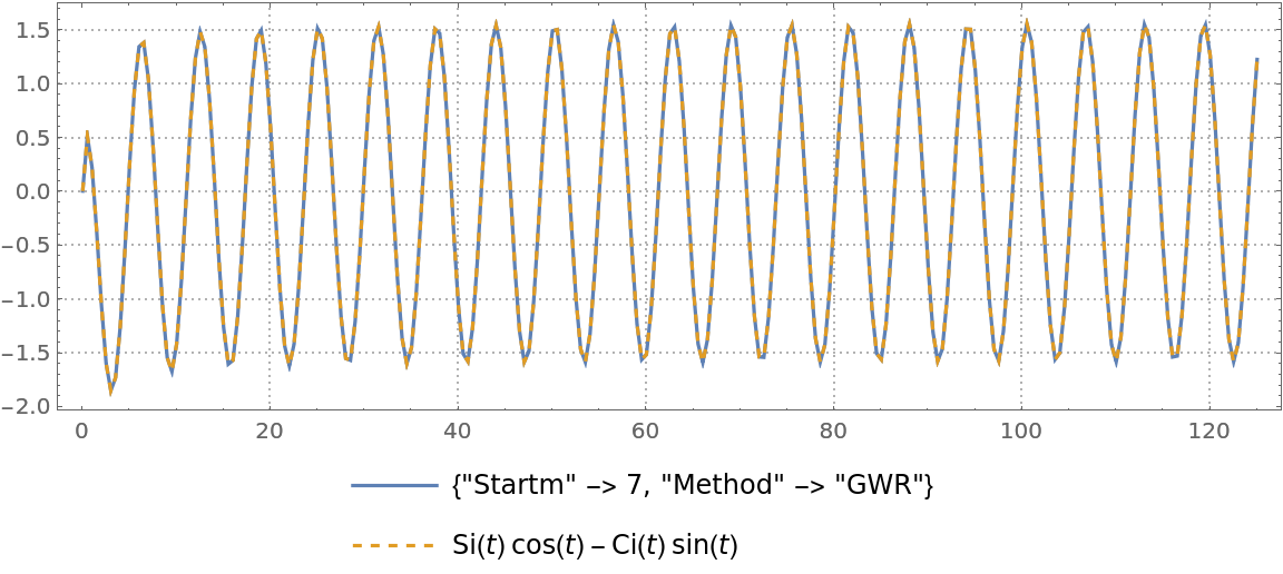
If we explicitly set the method to "FT", only that internal procedure will be called. The above problem can be solved with the default "Startm" if we specify "Method"→"GWR":
However, for significantly larger t-values, an elevated "Startm" is needed, regardless of the "Method" we specify. See additional remarks in the Author’s Notes.
Applications (2)
Find the maximum value and location of the inverse Laplace transform of example 2, first graphically and then using FindMaximum:
In the next application, we need to calculate average temperature. Assume that, solving a differential equation, we’ve obtained the following analytical result for the temperature as a function of time:
Symbolic integration is unable to calculate the average temperature in the time-interval between zero and one:
Now we try numerical integration with various options:
We see that numerical integration of this function is troublesome, so we recall that the Laplace transform of f7(t) is:
Using the operational rule for integration, the average temperature is:
Possible Issues (4)
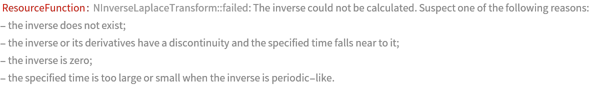
In this example, the expr is not a Laplace transform, and the inversion attempt fails:
For some Laplace transforms, a t-value that is too large (or too small) can be detrimental and will result in a failed inversion. Consider the transform of Sin(t):
A larger value of "Startm" will help, but it is better to avoid large t-s if the inverse is periodic:
The method fails in the vicinity points where the Laplace inverse, or its derivatives, have a discontinuity. In the following example at t=2, the third derivative of the inverse (the SawtoothWave function) has a discontinuity:
The following inverse has a discontinuity at t=25 and is zero for t<25:
Leaving out the Dirac delta component, the result of numerical inversion should agree with the simple expression:
Approaching from above with the numerical inversion, we can get quite near to the discontinuity (though with increasing computation time):
Numerical inversion works the best if the inverse transform is an analytic function.
Neat Examples (4)
Here, the result is a familiar number because the inverse transform is known to be Log(1+Sqrt(t)):
In this case the Laplace transform involves the MeijerG function (a rather complicated mathematical function that is nevertheless suitable for numerical evaluation in the Wolfram Language):
We can check symbolically that the result of the numerical inversion is correct:
Here, the inverse Laplace transform happens to be the two-parameter Mittag-Leffler function:
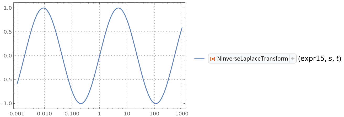
Here, the Laplace transform expression cannot be cast easily into a "real-only" form (though it is real for positive s-values):
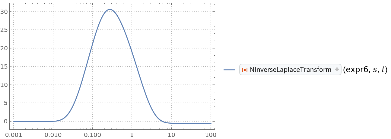
We prepare a log-linear plot:
The log-linear plot suggests that the inverse is simply Sin(Log(t)). A quick check proves the assertion:

![(* Evaluate this cell to get the example input *) CloudGet["https://www.wolframcloud.com/obj/e76a6b61-0b61-44ad-af0f-895d7468c2e4"]](https://www.wolframcloud.com/obj/resourcesystem/images/6d2/6d2b5ed0-6f57-431a-bdcd-54bc0310b330/18f486d760482c9d.png)
![expr6 = ((-1. + 100.*s)*
Sinh[0.5*Sqrt[s]])/(s*(Sqrt[s]*Cosh[Sqrt[s]] + s*Sinh[Sqrt[s]]));
LogLinearPlot[
ResourceFunction["NInverseLaplaceTransform"][expr6, s, t], {t, 0.001,
100.}, PlotRange -> All, PlotTheme -> "Detailed"]](https://www.wolframcloud.com/obj/resourcesystem/images/6d2/6d2b5ed0-6f57-431a-bdcd-54bc0310b330/0b788cac466d316a.png)
![Do[
{meth, NIntegrate[f7[t], {t, 0, 1}, Method -> meth]} // Print, {meth, {"GlobalAdaptive", "LocalAdaptive", "DoubleExponential", "MonteCarlo", "AdaptiveMonteCarlo", "QuasiMonteCarlo", "AdaptiveQuasiMonteCarlo"}}]](https://www.wolframcloud.com/obj/resourcesystem/images/6d2/6d2b5ed0-6f57-431a-bdcd-54bc0310b330/1a7f225a2a0453e7.png)
![Do[{t, ResourceFunction["NInverseLaplaceTransform"][Erf[5*Sqrt[s]], s,
t], f11[t], "Current time: " <> DateString["Time"]} // Print, {t,
25.1, 25., -0.02}]](https://www.wolframcloud.com/obj/resourcesystem/images/6d2/6d2b5ed0-6f57-431a-bdcd-54bc0310b330/79e35b5b180dde10.png)
![LogLinearPlot[
ResourceFunction["NInverseLaplaceTransform"][expr15, s, t], {t, 0.001, 1000.}, PlotRange -> All, PlotTheme -> "Detailed"]](https://www.wolframcloud.com/obj/resourcesystem/images/6d2/6d2b5ed0-6f57-431a-bdcd-54bc0310b330/1ffe8bc48aeae7c0.png)
![SeedRandom[1234]
Do[
tran = 10^RandomReal[{-2, 8}];
{tran, ResourceFunction["NInverseLaplaceTransform"][expr15, s, tran] == Sin[Log[tran]]} // Print
, 5]](https://www.wolframcloud.com/obj/resourcesystem/images/6d2/6d2b5ed0-6f57-431a-bdcd-54bc0310b330/058e05a9f8da3fc2.png)
![expr16 = Log[s]/(1 + s^2);
f16[t_] = Cos[t]*SinIntegral[t] - Sin[t]*CosIntegral[t];
tt = Range[0, 125, 0.5] + 0.001;
it = Table[f16[tr], {tr, tt}];
Do[ str = ToString[{"\"Startm\"" -> m, "\"Method\"" -> "\"Automatic\""}];
Row[{"Options:", str, " ", "start-time:", DateString["Time"]}, " "] // Print;
nt = Table[
NInverseLaplaceTransform[expr16, s, tr, {"Startm" -> m, "Method" -> "Automatic"}], {tr, tt}];
ListPlot[
{{tt, nt}\[Transpose], {tt, it}\[Transpose]}, Joined -> True, PlotStyle -> {Automatic, Dashed}, PlotRange -> All,
PlotLegends -> {str, f16[t]},
PlotTheme -> "Detailed", AspectRatio -> 1/3, ImageSize -> Large] //
Print;
Row[{"end-time:", DateString["Time"]}, " "] // Print;
Print[]; str = ToString[{"\"Startm\"" -> m, "\"Method\"" -> "\"FT\""}];
Row[{"Options:", str, " ", "start-time:", DateString["Time"]}, " "] // Print;
nt = Table[
NInverseLaplaceTransform[expr16, s, tr, {"Startm" -> m, "Method" -> "FT"}], {tr, tt}];
ListPlot[
{{tt, nt}\[Transpose], {tt, it}\[Transpose]}, Joined -> True, PlotStyle -> {Automatic, Dashed}, PlotRange -> All,
PlotLegends -> {str, f16[t]},
PlotTheme -> "Detailed", AspectRatio -> 1/3, ImageSize -> Large] //
Print;
Row[{"end-time:", DateString["Time"]}, " "] // Print;
Print[]; str = ToString[{"\"Startm\"" -> m, "\"Method\"" -> "\"GWR\""}];
Row[{"Options:", str, " ", "start-time:", DateString["Time"]}, " "] // Print;
nt = Table[
NInverseLaplaceTransform[expr16, s, tr, {"Startm" -> m, "Method" -> "GWR"}], {tr, tt}];
ListPlot[
{{tt, nt}\[Transpose], {tt, it}\[Transpose]}, Joined -> True, PlotStyle -> {Automatic, Dashed}, PlotRange -> All,
PlotLegends -> {str, f16[t]},
PlotTheme -> "Detailed", AspectRatio -> 1/3, ImageSize -> Large] //
Print;
Row[{"end-time:", DateString["Time"]}, " "] // Print;
Print[]; , {m, {5, 7}}]](https://www.wolframcloud.com/obj/resourcesystem/images/6d2/6d2b5ed0-6f57-431a-bdcd-54bc0310b330/080f46838befd327.png)