Wolfram Function Repository
Instant-use add-on functions for the Wolfram Language
Function Repository Resource:
Solve the linear minimax problem
ResourceFunction["LInfinitySolve"][m,b] finds an x that solves the linear minimax problem for the matrix equation m.x==b. |
Solve a simple minimax problem:
| In[1]:= |
| Out[1]= |
Create a 4×3 matrix, and b is a length-4 vector:
| In[2]:= |
Use exact arithmetic to find a vector x that minimizes ![]() :
:
| In[3]:= |
| Out[3]= |
Use machine arithmetic:
| In[4]:= |
| Out[4]= |
Use 20-digit-precision arithmetic:
| In[5]:= |
| Out[5]= |
Use a sparse matrix:
| In[6]:= |
| Out[7]= |
Here is some data:
| In[8]:= |
Find the line that best fits the data in the minimax sense:
| In[9]:= |
| Out[9]= |
Find the quadratic that best fits the data in the minimax sense:
| In[10]:= |
| Out[10]= |
Show the data with the two curves:
| In[11]:= |
| Out[12]= | 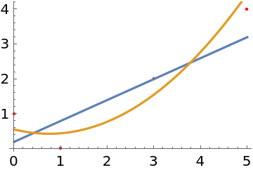 |
For a vector b, LInfinitySolve is equivalent to ArgMin[Norm[m.x-b,∞],x]:
| In[13]:= |  |
| In[14]:= |
| Out[14]= |
Create a 5×2 matrix, and b is a length-5 vector:
| In[15]:= |
Solve the minimax problem:
| In[16]:= |
| Out[16]= |
This is the minimizer of ![]() :
:
| In[17]:= | ![Show[Plot3D[Norm[m . {x, y} - b, \[Infinity]], {x, -2, 2}, {y, 0, 2}, MeshFunctions -> {#3 &}, ColorFunction -> (Hue[.65 (1 - #3)] &)], Graphics3D[{Red, PointSize[0.05], Point[{a[[1]], a[[2]], Norm[m . a - b]}]}]]](https://www.wolframcloud.com/obj/resourcesystem/images/623/6231f801-986a-497e-8b5a-b8f9e2341084/5a14edf6974755b0.png) |
| Out[17]= | 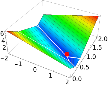 |
It also gives the coefficients for the line with minimax absolute deviation from the points:
| In[18]:= |
| Out[19]= | 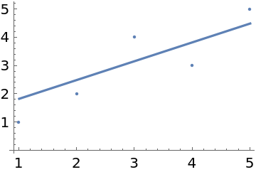 |
This work is licensed under a Creative Commons Attribution 4.0 International License