Wolfram Function Repository
Instant-use add-on functions for the Wolfram Language
Function Repository Resource:
Compute the Gromov–Hausdorff distance of finite metric spaces
ResourceFunction["GromovHausdorffDistance"][d1,d2] computes Gromov–Hausdorff distance of distance matrices d1 and d2. | |
ResourceFunction["GromovHausdorffDistance"][g1,g2] computes Gromov–Hausdorff distance of graphs g1 and g2. |
Gromov–Hausdorff distance of triangles in ℝ and ℝ2:
| In[1]:= |
| Out[1]= |
Gromov–Hausdorff distance of the star graph S3 and the cycle graph C3:
| In[2]:= |
| Out[2]= |
By[3], the path graph Pn and the circle graph Cn satisfy ![]() for all m,n and
for all m,n and ![]() for m>n. We can check this for small m and n:
for m>n. We can check this for small m and n:
| In[3]:= | ![ParallelMap[
ResourceFunction["GromovHausdorffDistance"][PathGraph@Range[2], PathGraph@Range[#]] &, Range[2, 6]]](https://www.wolframcloud.com/obj/resourcesystem/images/5d5/5d5714dc-be26-479a-891d-d4ff51cecffa/043c71e7fb744cb3.png) |
| Out[3]= |
| In[4]:= |
| Out[4]= |
Note that dGH(G1, G2) = 0 if and only if G1 and G2 are isomorphic.
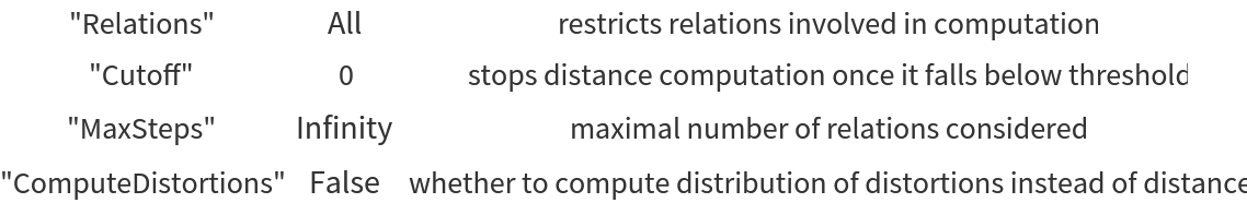
Taking into account only the "Minimal" possible relations with max(n1, n2) elements is often sufficient:
| In[5]:= | ![ParallelMap[
ResourceFunction["GromovHausdorffDistance"][CycleGraph[3], CycleGraph[#], "Relations" -> "Minimal"] &, Range[2, 6]]](https://www.wolframcloud.com/obj/resourcesystem/images/5d5/5d5714dc-be26-479a-891d-d4ff51cecffa/13d152ed53a0c24a.png) |
| Out[5]= |
Considered relations can be specified by their size:
| In[6]:= |
| Out[6]= |
Setting a "Cutoff" provides an upper bound on the Gromov–Hausdorff distance:
| In[7]:= |
| Out[7]= |
Computation stops after the maximal number of relations has been processed:
| In[8]:= |
| Out[8]= |
Count how many relations yield each pair {dist,k}:
| In[9]:= |
| Out[9]= |
Wolfram Language 13.0 (December 2021) or above
This work is licensed under a Creative Commons Attribution 4.0 International License